OpenDCS Computations - Introduction

OpenDCS includes a program called Computation Processor. This tool is used for creating computations on the data stored in the time-series database. It is currently supported for the U.S. Bureau of Reclamation Hydrologic Database (HDB)and the U.S. Army Corps of Engineers Corps Water Management System (CWMS).

Recall that once the Computation Processor is launched (launcher_start.bat), users must log-in with the following credentials.

USACE users:

• USERNAME: Username

• PASSWORD: Oracle

Computations can be helpful for operations because of the following abilities:

• Automate calculations

• Transform time series to another interval or period

• Calculate sum or average over a period

• Transform one parameter to another parameter

• Create and employ customized algorithms

How to Set-Up a Computation in OpenDCS?

In OpenDCS, a computation comprises of a few pieces:

• Algorithm (ie operations applied)

• Input & Output Time Series or Pathname Parts

• Process

• Optional - Group

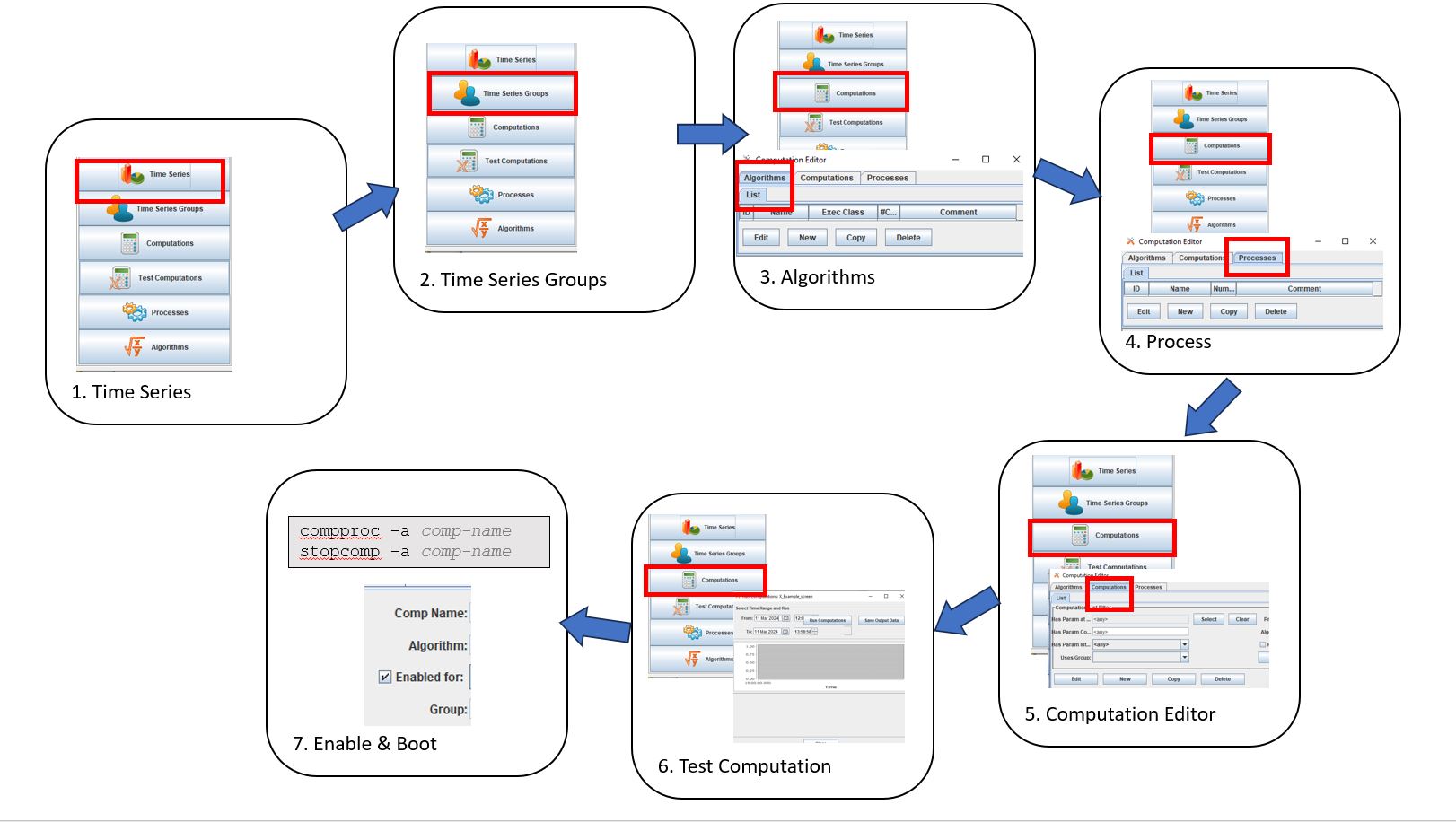
A suggested guiding principal to building a new computation is to follow the steps outlined below:

1. Ensure input time series exist

2. Create group if computation is going to be applied to multiple time series

3. Ensure algorithm exists (create if necessary)

4. Ensure process exists

5. Create computation

6. Test computation

7. Enable computation

The next steps outline an example for putting together a very simple “calculation” using the computation processor. The steps are intended to provide a template for how to set up a computation and familiarize a user with the tabs and tools needed to get started. Some steps are assumed already completed but will be touched upon.

At the end of this section, a user should know how to set up a calculation that grabs the top of hour value from a higher resolution time series and creates a new hourly time series. In this example, the higher resolution time series will be six minute data.

1.Time Series Check

The first step to setting up a calculation is knowing the path name parts to the time series and ensuring the time series has data populated.

As a recap, time series have 6 parts.

location.param.statcode.interval.duration.version

or

location.param.paramtype.interval.duration.version

Note - the location, param, and version parts are often subdivided with hyphens. See section Time Series Introduction for more details on time series.

• location - This refers to a Site in the database. This is the site name.

• param - This is the Data Type (such as precip, stage, speed, etc).

• statecode or paramtype (such as ave, inst, max, min, total).

• Interval (0, 15 min, 1 hour, 1 day, ~ 1 month, ~ year)

• Duration (0, 1Hour, 1Day, 1Month, 1Year)

• Version (meta data such as data steward or raw/revised status)

2.Time Series Groups

If you plan to use the same algorithm on similar time series multiple times, it is recommended to use OpenDCS Time Series Groups. This tool is quite simple. It is a way to name a group of time series and call it when setting up a computation. Typically, time series are grouped by “region”, “basin”, “data-type” or “site-group”.

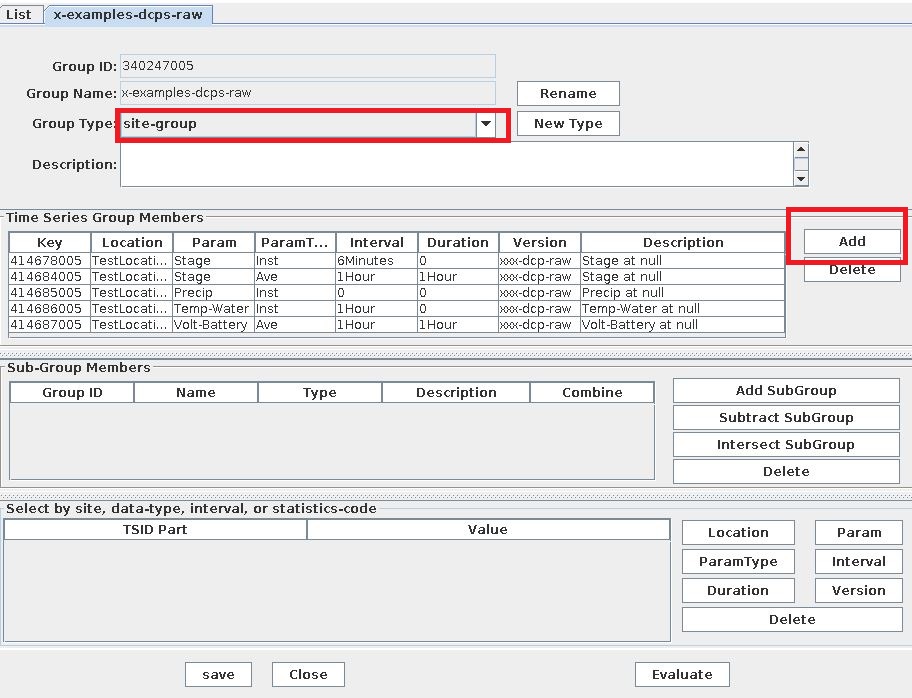
To edit groups, launch the “Time Series Groups” application from the main menu. Click on the button at the bottom of the window “New”.

A small window will pop up to name the group. Enter a name. Note that this name can be edited after creation using the “rename” button displayed in the image below.

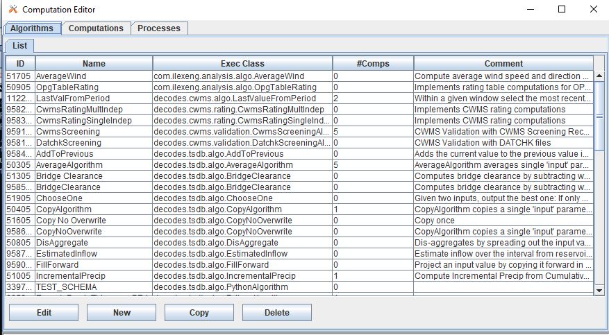
3.Algorithms Intro

The Algorithms tab in the Computations Editor is where default Computation Processor algorithms are stored, in addition to custom algorithms added by users. Algorithms, in OpenDCS, can be thought of as instructions or like a function that has yet to be called or invoked. Examples of default algorithms are listed below:

• Copy

• IncrementalPrecip

• Sum

• Average

• USGS

• Screening

4.Process Intro

Processes are a way of grouping computations together to help spread the computational load of the system. Once a computation is created, it can be attributed to a process.

Creating processes can also be beneficial because of their ability to reduce operational run time, reduce backfilling run time, and help maintain and organize computations.

To create a new process, follow one of the following steps:

#. Launch the Process Monitor by clicking the “Processes” button from the main menu. To add a new process click “New”. #. Launch the Computations Editor and navigate to the “Processes” tab. To add a new process click “New”.

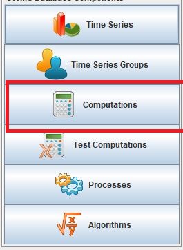
5.Computation Editor Intro

Once algorithms and processes are defined, now a user is ready to set up a computation. On the “Computations” tab of the Computation Editor. The editor will display a few items, including the computation Name, Algorithm used in the Calculation, the Process for which the computation is applied, and the status of whether the computation is enabled.

If there are already a number of computations in the editor list, the top portion of the screen can be used to filter computations by some time series parts or groups.

The following examples outline how to set up a few basic introductory computations. This means that the computations employ simple to understand algorithms, are common in practice, and demonstrate the nuts and bolts of using the computation processor.

In the examples below, all the time series and computations are in UTC. In most cases the examples below show how the default output is calculated. For more information about how to apply time shifts, and manipulate the calculation.

To create a new computation click on the “New” button on the bottom of the “List” tab. A window will pop up instructing the user to enter a name. Note that any name entered here can be edited once it is created. Best practices suggest that the name specify some information that easily conveys what type of time series is or are being calculated.

Once the name is entered and saved (click “OK) then a window will pop up for the computation. Generally the window for each computation will include a top section which is where users can specify the algorithm used in the calculation, change in the name of the computation, apply the process, and call a group for the computation (if applicable). Users can also specify a start and end time for when the computation is effective. Recall that by default, computations in the computation process are triggered when new data is available in the database.

For more information about the default or standard algorithms that come installed in OpenDCS see Resources - Algorithms.

Sample Calculation: Copy Time Series

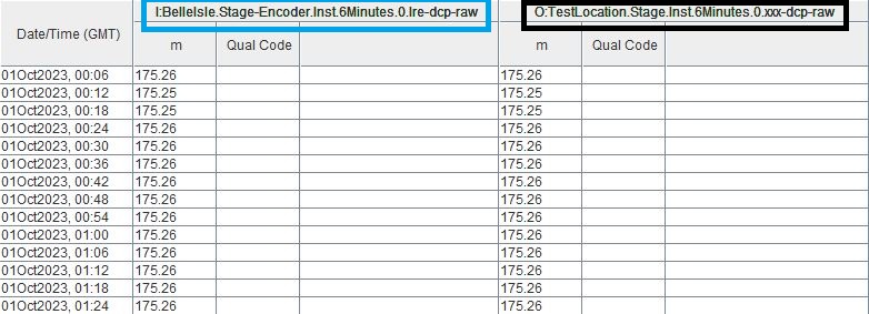
In the following example, the computation is a direct copy of the data in the time series path. See in the image below the left hand side is the input denoted with “I” and the right hand side is the output denoted with “O”. The image is from the “Run Computation” button, which will be elaborated on in the Test Computation section below.

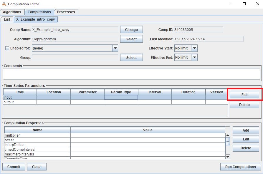
After the computation is named, the following window will pop up.

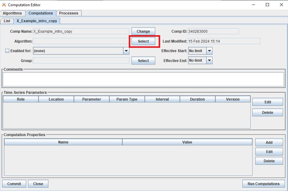
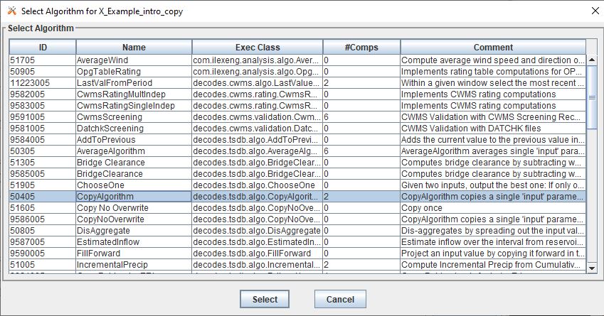
After the computation is created, select the algorithm by clicking the “Select” button next to the Algorithm section. A window will pop up with a list of the available algorithms. Select the CopyAlgorithm.

Once the algorithm is selected, the Computation Properties section at the bottom of the window will populate with some Names and the Values will be blank.

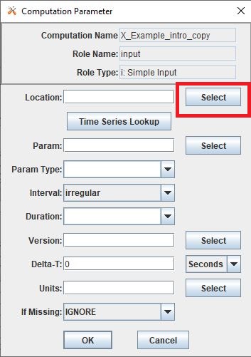
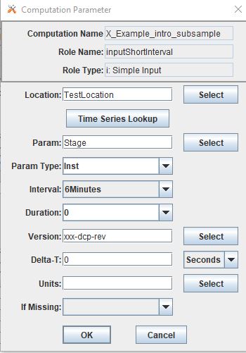
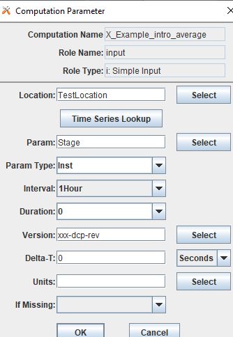
Additionally, two rows will populate in the Time-Series Parameters section: and input Role and and output Role. Select either of the roles and click “Edit” on the right. And the following window will pop up for the user to enter specifics about the input time series for which the algorithm should be applied.

In this example, the existing time series is:

BelleIsle.Stage-Encoder.Inst.6Minutes.0.lre-dcp-raw

To select this time series as the input and populate the window, click the “Select” on the right of the Location box, and select the location of the input time series.

Once the Location is selected, users can either manually enter the corresponding time series parts below, or use the “Time Series Lookup” to view existing time series for the location selected.

Once the time series is selected, the parts will populate.

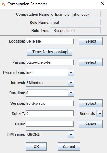
NOTE - by default the following parameters are:

• Delta-T 0 seconds (more details are in the resources section)

• Units empty (by default the units will be the original units of the time series)

• If Missing IGNORE (if the input value is missing, the calculation will not be executed)

Click “OK” and then select and edit the output time series parameter. In the “Edit” output parameters enter the time series parts for which the desired output will consist of.

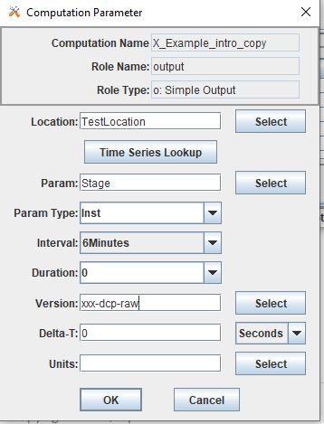
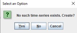
If it the time series does not exist yet, a box will pop up prompting the user to allow the creation of the desired time series. Click “Yes”. Or if there is something that needs to be modified, click Cancel and correct.

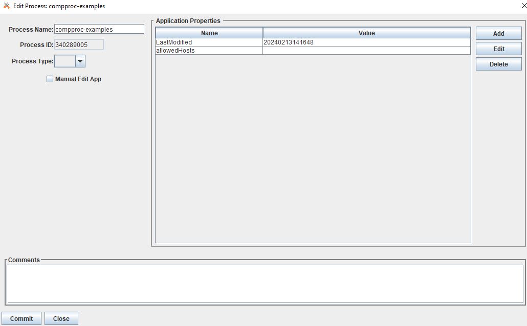
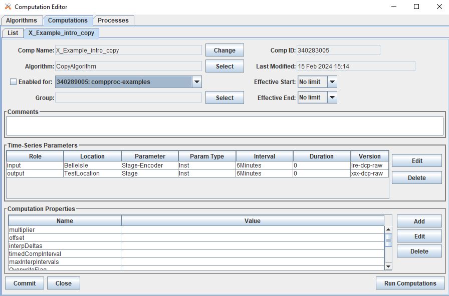
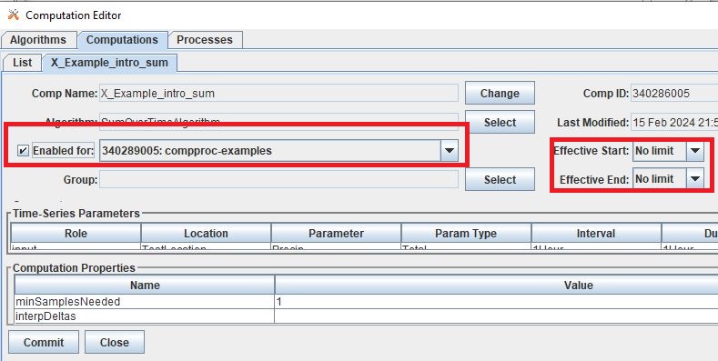
As a last step, select the process for which this computation will attributed to. Do this by selecting the drop down menu next to the “Enabled for” box. Select the process.

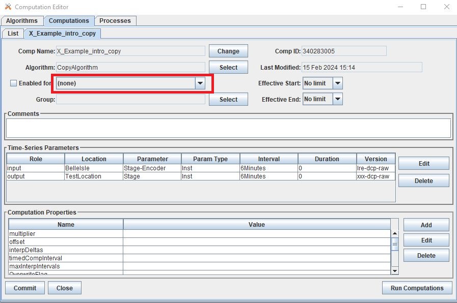
In the example below the process compproc-examples is selected.

As a final few steps - add in any comments about the computation for documentation purposes. Click “Commit” on the bottom of the screen so that all the steps above are saved.

Sample Calculation: Stage - Top of Hour

In the following example, the computation uses the SubSample algorithm to extract the top of hour values from a higher resolution time series. In this example the input time series consists of 6 minute data. The image below is from the “Run Computation” button, which will be elaborated on in the Test Computation section below.

The following image shows how the computation should be set up. Once the SubSample algorithm is selected the Computation Properties at the bottom of the screen will populate with some default settings.

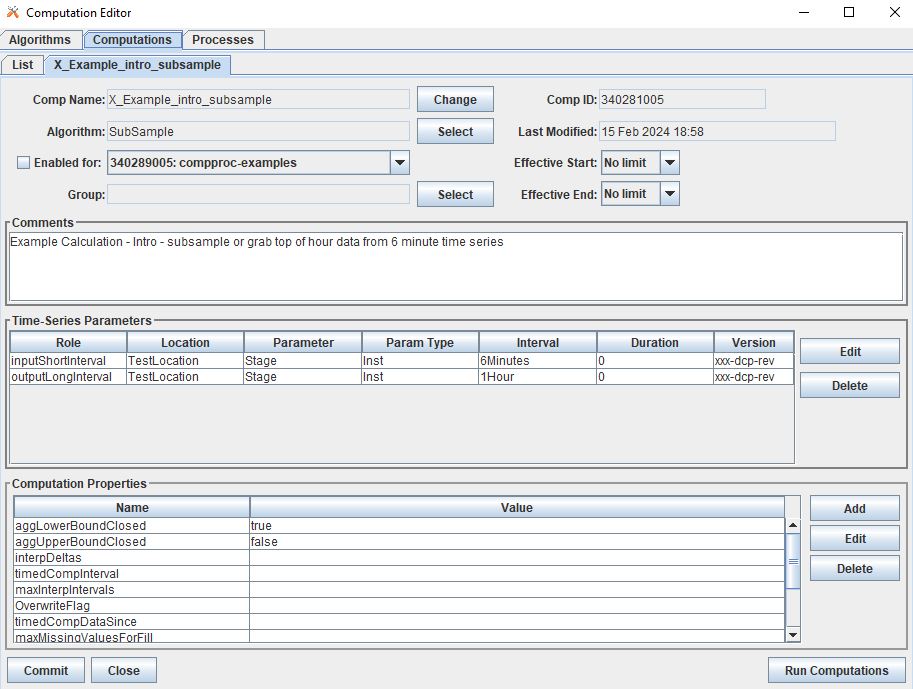
• aggLowerBoundClosed : true

• aggUperBoundClosed : false

The input and output roles for this algorithm are called

• inputShortInterval: the input time series which is a higher resolution time series than output

• outputLongInterval: the output time series which is a lower resolution time series than input

By default in this computation the “If Missing” is set blank.

Sample Calculation: Stage - Daily Average

In the following example, the computation uses the AverageAlgorithm algorithm to calculate a daily average based on hourly inputs. In this example the default computation properties are used. This includes the current default property that the minimum input samples needed for the calculation to run is 1. No time shifts or adjustments of any kind are applied. The image below is from the “Run Computation” button, which will be elaborated on in the Test Computation section below.

The following image shows how the computation should be set up. Once the AverageAlgorithm algorithm is selected the Computation Properties at the bottom of the screen will populate with some default minSamplesNeeded. The input and output roles are:

• input:

• average:

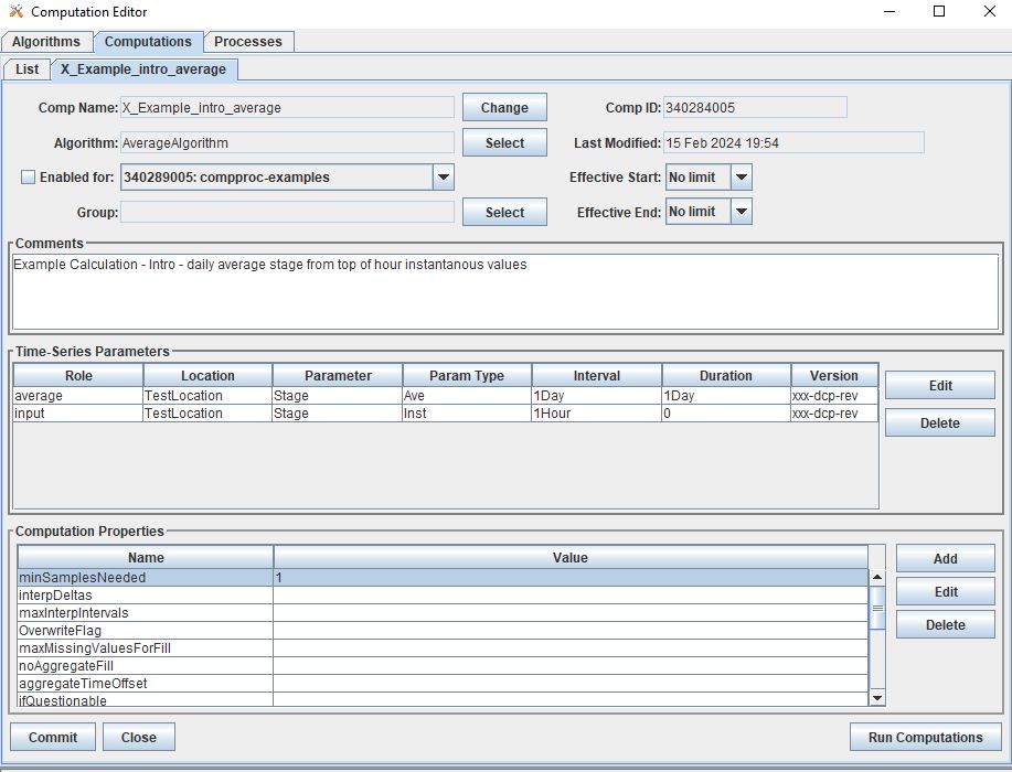
By default in this computation the “If Missing” is set blank.

By default, the average will use the lowest bound and upper bound. For daily averages, this means the average will use hours 00-23.

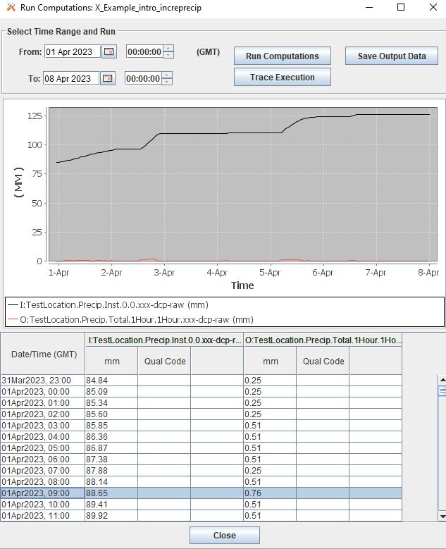
Sample Calculation: Precipitation - Cumulative to Incremental

In the following example, the computation uses the IncrementalPrecip algorithm to calculate hourly precip totals from a cumulative precip time series with cumulative totals recorded every hour. Put simply, the function calculates the difference between the intervals defined in the output time series. This example includes the default properties for the computation. The image below is from the “Run Computation” button, which will be elaborated on in the Test Computation section below.

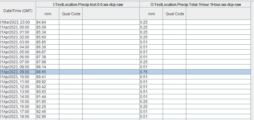
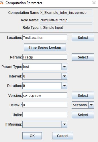
The following image shows how the computation should be set up. Once the IncrementalPrecip algorithm is selected the Computation Properties at the bottom of the screen will populate with default aggLowerBoundClosed and aggUpperBoundClosed as true. The input and output roles are:

• cumulativePrecip (input): cumulative precip time series

• incrementalPrecip (output): output time series

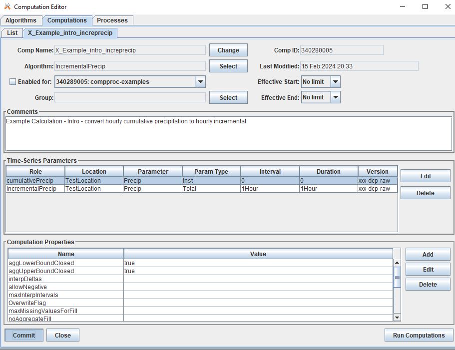
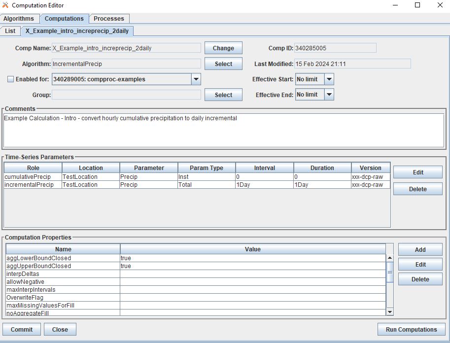
By default in this computation the “If Missing” is set blank.

Define the output time series based on the intervals and duration desired.

The output will calculate the difference between the current time step and the next time step, so long as the value is not negative.

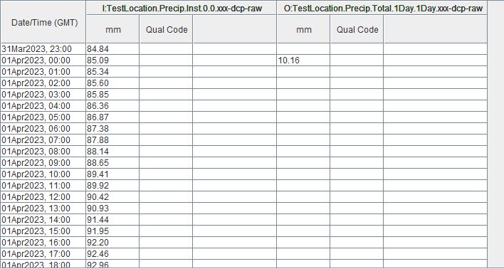
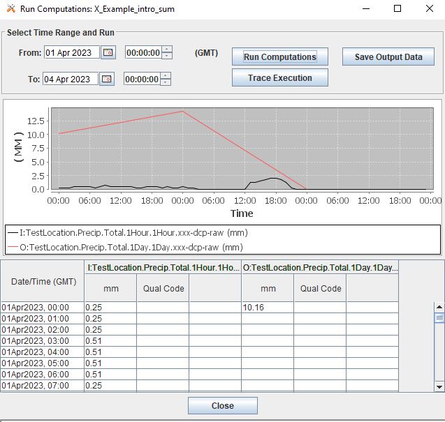
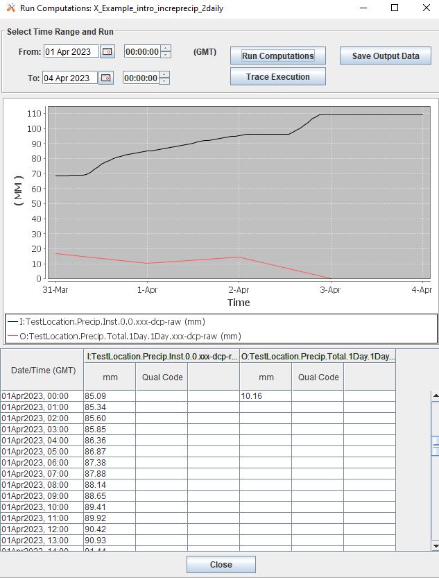
Sample Calculation: Precipitation - Daily Total

The following example is intended to demonstrate how the “SumOverTimeAlgorithm” can be used to sum up incremental precipitation, if the most raw data is provided as incremental. If the cumulative hourly time series is available, it is best practice to use this time series as the input, as opposed to calculating the hourly incremental totals and then summing over the incremental totals.

6.Test Computation Intro

Once a calculation is set up, like any of the examples above, users can test or run the computation to check and verify that the computation is calculating the desired output correctly.

To test or run a computation, simply open the computation from the List. To open the computation from the List, select the desired computation, and click “Edit” on the bottom of the page.

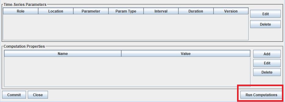
Once Run Computations is launched, a window will pop up with a top pane that shows an empty graph area with Time on the X-axis. To run a computation, define the time window. If the input data is a high resolution, good practice is to start with a small time window range to reduce the run time. Once the calculation has been verified, then increase the time range.

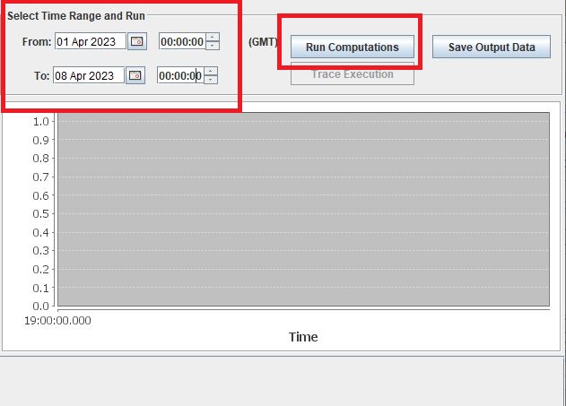
Dates and Times can either be selected using the small calendar icon or by manually entering in the date in form “DD MMM YYYY”.

Click “Run Computations” and if the output looks correct, then save the output if the user wished to save the output. To save click “Save Output Data”.

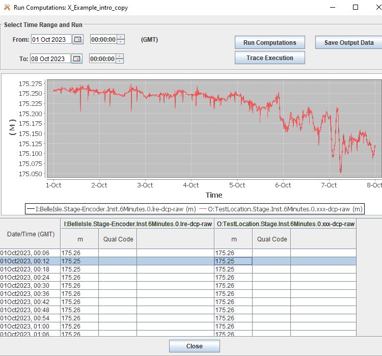
Run Calculation: Copy Time Series

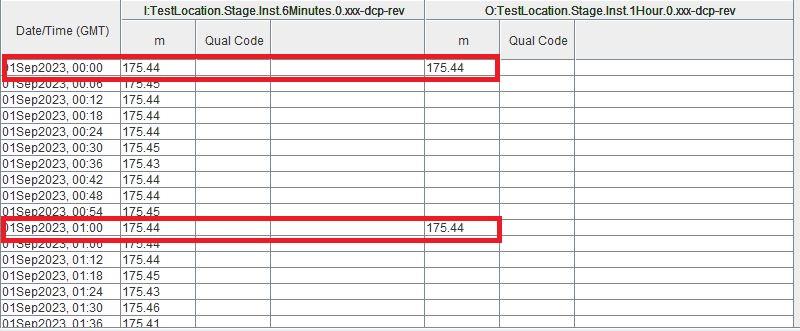
The example outlined above for copying a time series using the Computation Processor is demonstrated in the following window. The output line (red) covers directly over the input line (black).

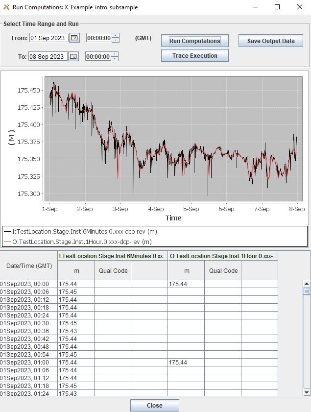
Run Calculation: Stage - Top of Hour

The example outlined above for sub sampling the top of the hour is demonstrated in the image below.

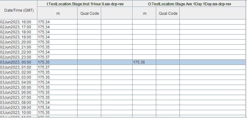
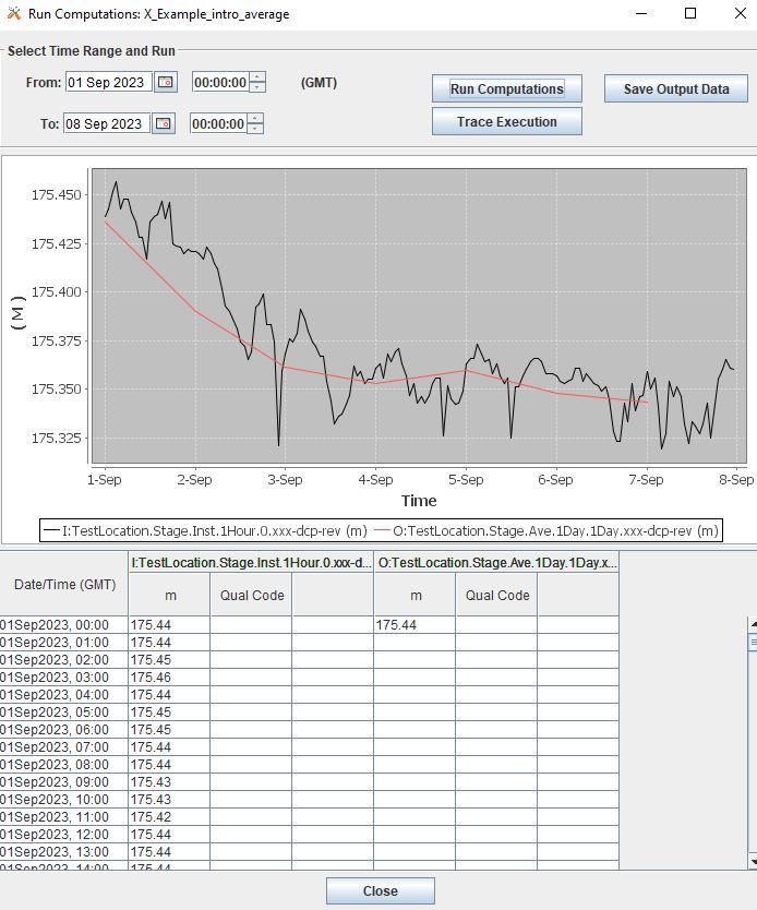
Run Calculation: Stage - Daily Average

The example outlined above for calculating a daily average from hourly values is demonstrated below.

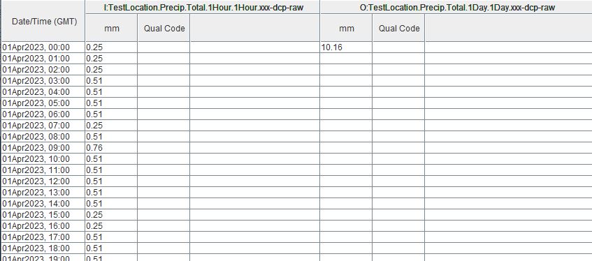
Run Calculation: Precipitation - Cumulative to Incremental

The example outlined above for calculating hourly incremental precipitation totals from cumulative hourly precipitation is demonstrated in the graphic below.

Run Calculation: Precipitation - Daily Total

There are two methods for calculating the daily total. One method is to sum the hourly totals that are calculated in the previous example. The other method is to use the incremental precipitation algorithms, but change the increments and duration in the output time series. The two methods are displayed below. It is good practice to use the raw original data as the input rather than adding in extra calculations and steps that can potentially accrue small erros.

7.Enable & Boot Intro

Once the computations are set and tested for accuracy, then the computations can be set to run automatically. This means that the calculations will by default be triggered for a time increment for which the input time series has new data for such time increment. To clarify, this means that computations are not going to be run for the entire time series period of record. Rather computations are only going to be run for periods for which there is new input data.

Users can opt to define an Effective start and end date. This can be beneficial to help users avoid accidentally triggering calculations for very long periods of record. It is unlikely to occur, however, when such a que of calculations is triggered, depending on the resolution and number of processes defined, the run time can slow down calculations and in some cases take some time to backup.

To enable a calculation, check the enabled box, and make sure the process defined above is selected. Define any effective start or end dates. Click Commit to save changes.

Once the computation is created and saved and enabled, it needs to be added to the computations daemons to run in the background. For example, the following line should be added to any Boot or Start script for the computations to be fully enabled.

compproc -a compproc-examples

Until such process is added to a boot script the computations will not be run automatically. However, a user can always run them from the GUI, as demonstrated in the previous section.

To stop a process add the following to a Stop or Off script.

stopcomp -a compproc-examples

More about Computations

The steps above outline a few simple computations, set-up using default settings in algorithms and computations. The Computation Processor includes a set of tools that can be used to create more complex algorithms or computations, including some of the following:

• Time shifts

• Minimum criteria

• Redefining floor/ceiling criteria

• Defining trigger input criteria

• Writing custom algorithms that pull data from the database