Computation Processor User Guide

This Document is part of the OpenDCS Software Suite for environmental data acquisition and processing. The project home is: https://github.com/opendcs/opendcs

See INTENT.md at the project home for information on licensing.

Overview

The Computation Processor is a suite of programs for executing computations on data stored in a time-series database. It is currently supported for the U.S. Bureau of Reclamation Hydrologic Database (HDB) and the U.S. Army Corps of Engineers Corps Water Management System (CWMS, pronounced ‘swims’).

The CP is designed to handle many types of computations:

• USGS Rating Algorithm: Table lookup with shifts.

• Consumptive Use = Subtract return flow from diversion.

• Periodic averages, minimums, maximums, and other statistics

• Total flow at several stream gages to calculate reservoir inflow.

• Variation on total flow: gages could be far upstream, allow a time-offset on each gage. Note that this could result in future (forecasted) flows.

• Reservoir surface elevation = gage height + base elevation.

• Total reservoir release = bypass releases + turbine releases + spill.

• Cumulative annual precip = previous value plus delta from recording device. Omit negative deltas (which would mean the device was reset).

• Percent of normal precip = specified year’s cumulative annual precip / cumulative annual precip averaged for number of years.

• Polynomial with constant or seasonally-changing coefficients.

• Interpolate between two other computations. Example: transition from one rating to another

• 3D Table Lookup: Two input parameters, one output parameter.

A composite computation might also be defined that combines several of the above primitive types. The CP is packaged with the following components:

• Generic Time Series Database Interface with extensions to support USBR (U.S. Bureau of Reclamation) HDB (Hydrologic Database), and USACE (U.S. Army Corps of Engineers) CWMS (Corps Water Management System).

• DECODES Consumer to ingest incoming DCP (Data Collection Platform) data and store it directly into either HDB or CWMS.

• The background Computation Processor that watches the database for incoming data and performs computations as needed.

• An initial set of algorithms (periodic averages, adding & scaling, stage to flow conversions with USGS RDB files, deltas).

• GUI (Graphical User Interface) editors for computational meta-data and Java algorithms.

• XML (Extensible Markup Language) Import and Export utilities for archiving and transferring computational meta-data.

• This manual.

The CP is designed for flexibility in several ways:

1. The GUI algorithm editor makes it is easy to add new types of algorithms without an expert-level understanding of Java.

2. The database interface is designed to work with any SQL DBMS.

3. The data structures and operational concepts are designed to accommodate HDB, NWIS, CWMS, and Sutron’s commercial Tempest Hydro-Met Analysis product.

The last item requires some elaboration:

Funding for the CP was provided by USBR, USGS (U.S. Geological Survey), and USACE. We initially developed and tested the code against USBR’s Hydrologic Database. Sutron has used it extensively within their Tempest™ Hydro-Met Analysis product for derived parameters and limit-checking. In 2008 and 2009 it was ported to work with USACE’s CWMS database. Thus the CP is currently operational in 3 different database systems, each with different schema.

Glossary and List of Acronyms

CP Computation Processor – the background program that executes computations as new data arrives.

CCP CWMS Computation Processor – i.e. the CP configured for CWMS.

CWMS Corps Water Management System (pronounced ‘swims’) - A system for hydrologic data storage and analysis used by USACE.

DBMS Database Management System

DCP Data Collection Platform – equipment in the field that collects and transmits raw environmental measurements.

DECODES DEviceCOnversion and DElivery System – A collection of software for decoding raw environmental data, and converting it to a time-series in a variety of formats.

ERD Entity Relationship Diagram

GUI Graphical User Interface

HDB Hydrologic Database – A system for hydrologic data storage an analysis used by USBR.

NWIS National Water Information System - A system for hydrologic data storage an analysis used by USGS.

SDI Site Data-type ID. In HDB this is used to denote a particular parameter at a particular site. It is stored as a numeric ID.

SQL (a.k.a. “sequel”) Structured Query Language

TSDB Time Series Database

USACE U. S. Army Corps of Engineers

USBR U. S. Bureau of Reclamation

USGS U. S. Geological Survey

XML Extensible Markup Language

Theory of Operation

Figure 1 shows the workflow for the CP. The “Computation Processor Application” is a Java program that runs continually in the background.

• It is triggered when new time-series data arrives in your database.

• The program finds all computations that you have defined that depend on the new data. Computations are defined in special tables within the database.

• The program attempts to execute these computations, which may involve retrieving other data from the database. For example, if the computation is to add A and B, when a new value for ‘A’ arrives, we may need to fetch a previously stored ‘B’ value.

• Results are written back to the time series database. This may (as is the case for HDB) trigger an external database QC process.

• When results are written, this may recursively fire other computations, and so on.

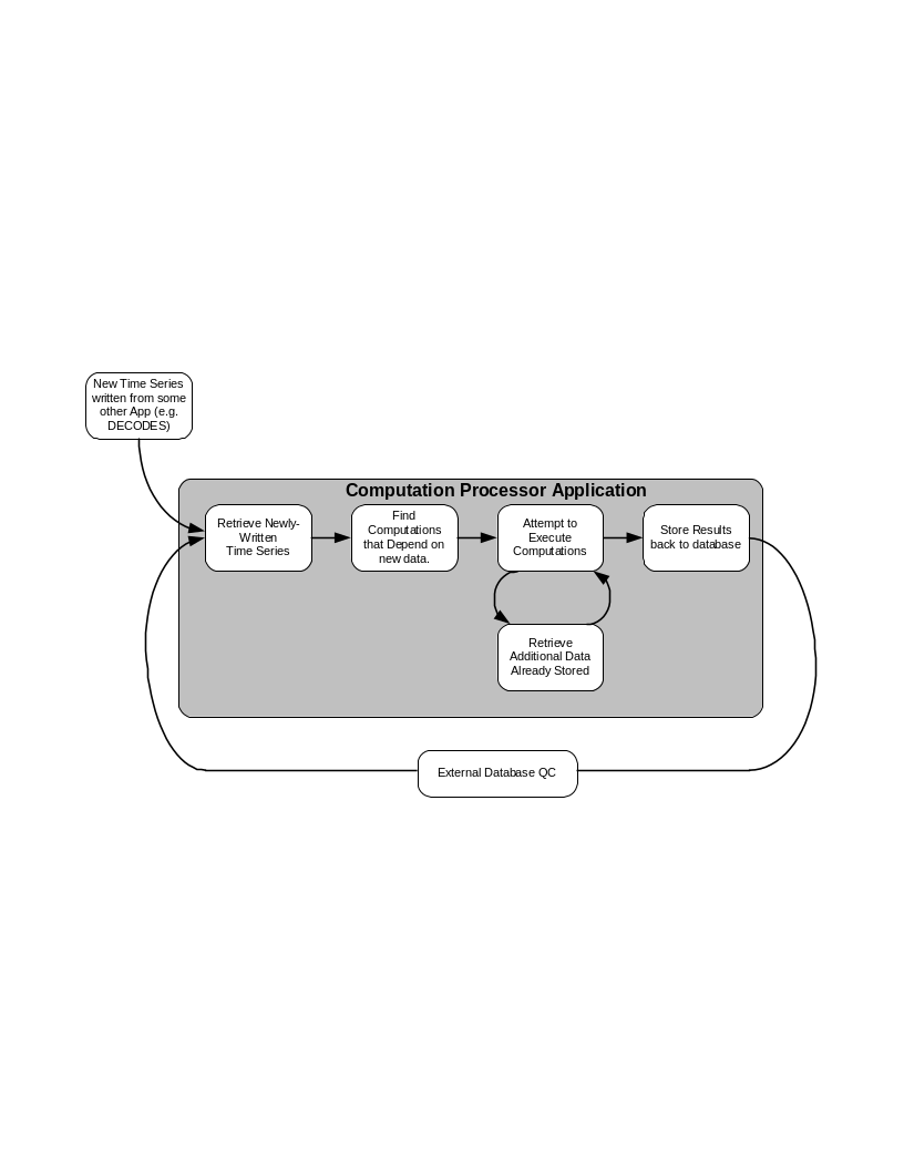
Figure 1: Workflow for the Computation Processor.

Time Series Database Assumptions

The CP assumes that you are storing hydro-meteorological data in a SQL database. We have striven to isolate the code that accesses the database into a few classes with abstract Java interfaces. The goal is to make it as easy as possible to adapt CP for many organizations.

The CP makes several assumptions about how data is stored in the time-series database:

• Sites represent locations and each site has a unique string ID.

• Data type codes are used

• USGS uses numeric EPA codes.

• HDB uses its own numeric codes.

• CWMS uses standard 2-part string codes like “Stage-Pool”.

• Many other agencies uses SHEF physical element codes.

• A particular parameter at a particular site can be denoted by a single numeric ID called a SDI (for Site Datatype ID).

• For HDB this is called the SDI.

• For NWIS this is called a Data Descriptor ID.

• For CMWS this is called TS_CODE.

• The database may store parameters of different intervals in different tables.

• HDB has INSTANT, HOUR, DAY and other tables.

• USGS NWIS has Unit value tables, Daily value tables and others.

• CWMS many interval codes including: 1Minute, NMinutes (where N can be 2, 3, 4, 5, 6, 10, 12, 15, 20, or 30), 1Hour, NHours (where N can be 2, 3, 4, 6, 8, or 12), 1Day, Week, 1Month, 1Year, 1Decade.

• An additional string element called a “table selector” can be used to build part of the table name that stores a particular parameter.

• For HDB this is a prefix denoting real (R_) or modeled (M_) data.

• For USGS this is a function of the database number (DBNO).

• For CWMS this provides the remaining parts of the 6-part DSS path name.

CP and DECODES Mapping to HDB

The CP and DECODES were designed to cross-platform. Generic concepts are mapped to HDB in the following ways:

Sites represent locations and each site has a unique string ID. Entities in the HDB_SITE table are mapped to Site objects in CP and DECODES. The numeric site ID appears as the “hdb” site name type. In Figure 2, note the different name types. Also note the “hdb” column containing the numeric IDs.

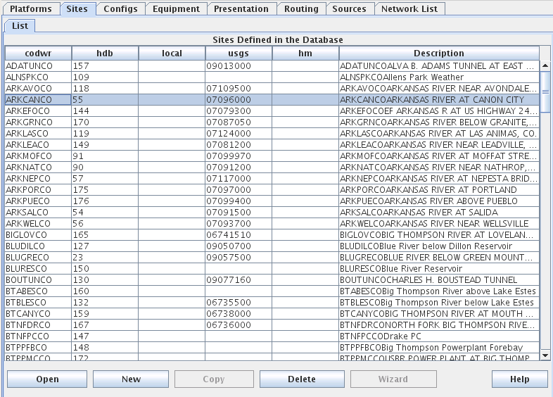
Figure 2: Site List Tab in DECODES Database Editor (dbedit).

You can add/remove site name types for your system with the “rledit” (Reference List Editor) command.

Figure 3 shows the reference list editor. There are many “Enumerations” that you can modify in this GUI. After making changes select File – Save to DB to make your changes permanent.

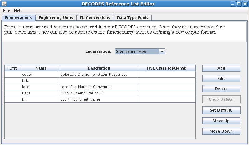
Figure 3: Reference List Editor being used to modify the Site Name Type Enumeration.

DECODES and CP support Data Type codes from multiple standards. HDB uses its own numeric codes. USGS uses numeric EPA codes. CWMS uses standard 2-part string codes like “Stage-Pool”. Many other agencies use SHEF physical element codes.

In DECODES Sensors, you can control this directly by entering multiple data types for each sensor.

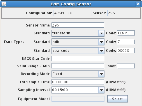
Figure 4: DECODES Edit Sensor Dialog, showing multiple data type codes.

DECODES can also attempt to automatically translate between data coding systems. The “Data Type Equivalence” tab of the rledit program is shown in Figure 5. If you share DECODES configurations with other agencies in your area (for example Colorado Division of Natural Resources uses a data type coding system called “transform”), you may add their coding system and establish equivalences to HDB data types.

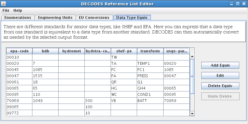
Figure 5: Reference List Editor - Data Type Equivalence Tab.

To establish a new coding system:

• On the “Enumerations” tab, select the “Data Type Standard” enumeration and click the add button.

• Click File – Save to DB.

• Exit the rledit program and restart.

• On the “Data Type Equiv” tab, use the buttons at the right to add, edit, or delete equivalences to HDB data types.

For your computations, you will always want to enter the numeric HDB data type.

In HDB, the SDI (Site Data-Type ID) is used to combine the numeric site and data type IDs into a single integer. This detail is usually invisible to the user but occasionally shows up in error and log messages.

A string element called a “table selector” is used to denote real (R_) verses modeled (M_) data.

Computation Meta-Data

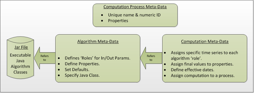
Figure 6: Logical Depiction of Computations Meta Data.

The above diagram illustrates the types of information used to execute computations.

In the lower right, we see “Jar File”. JAR stands for Java Archive. Java software is distributed as one or more jar files. You will need these jar files:

• decodes.jar (included in OPENDCS release. This is found in the “bin” directory under the installation. This file contains all of the code for DECODES, the CP infrastructures, and the built-in algorithms.

• ojdbc14.jar (provided by Oracle). This contains code that allows CP to talk to an Oracle database. It is not included in the release. You must place it in the “dep” directory under the installation.

• Algorithm-JARs: If you create your own algorithms, you should place them in the “dep” directory under the installation.

• You may also define the environment variable CP_SHARED_JAR_DIR pointing to a directory containing JAR files that you want to be shared. These jars will be included in class path ahead of the ones in the dep directory.

At the top we see “Computation Process Meta Data”. The database defines “loading applications” for any application that can load time-series data into the database. You can see all of the loading application in the “compedit” (Computation Editor) program, on the “Processes” tab. We define the following loading applications:

• DECODES – for DECODES routing specifications that load raw time-series data from incoming DCP messages.

• compproc – The background computation process daemon.

• compedit – the computation editor

• runcomp – the GUI for interactively running computations

• compdepends – the background process that maintains

• compproc_regtest – This is not required for all installations. It is used for running the regression tests only.

An Algorithm is an abstract set of instructions for performing a particular type of computation. Examples would be “periodic average” or “USGS Rating Table Lookup”. Each algorithm has a CP_ALGORITHM record containing the name of the Java class that will execute the computation. You can see all of the algorithms defined in compedit, Algorithms tab.

• Algorithms have one or more time-series parameters (CP_ALGO_TS_PARM). These denote the inputs and outputs of the algorithm. Each parameter has a ‘role name’ denoting how it is used within the algorithm.

• Algorithms also may have one or more named properties. These are used to control various aspects of the algorithm. For example, a rating table algorithm might have a property denoting the directory in which to find rating table files.

A Computation applies an algorithm to specific parameters in the time series database. It is assigned to be executed by a particular loading application.

• The CP_COMPUTATION record associates a computation with an algorithm and a loading application.

• Computations may only be valid for a certain time period, denoted by the effective start and end times in the record.

• There will be a CP_COMP_TS_PARM record corresponding to the algorithm parameter records (CP_ALGO_TS_PARM). This is where a specific SDI, interval, and table-selector are assigned to the algorithm’s roles.

• A ‘Delta-T’ value may optionally be assigned. This allows us to correlate data values at different times. For example, suppose we are adding two inflows from different streams, and that the gage for one stream was 3-hours upstream.

• A computation may also assign values to the algorithm’s properties. This is done with a CP_COMP_PROPERTY record.

A Time-Series Group is a flexible way of defining a group of time-series that share some attribute. For example you could have a group of all “Stage-Tail” values with Version “raw”. Groups are important for reducing the number of computations you have to maintain. For example, if you have the same set of 5 computations that you execute on all Stage values. You can just define a group of these time-series and use it as input for the 5 computations. You don’t need to redefine the computation for each site.

Computations Meta-Data ERD

The following figure shows computation meta-data as it is defined in the HDB database.

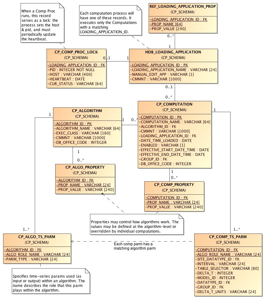
Figure 7: Computation Meta-Data Entity Relationship Diagram (ERD).

Tools Provided with the CP

Figure 8 shows how the tools interact with each other and the time series database. For completeness we also show some of the DECODES tools which process raw data as it arrives from the field.

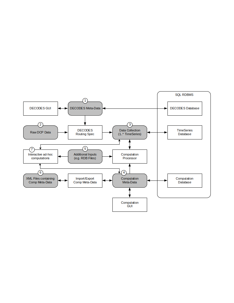
Figure 8: Workflow through the Provided Tools.

1. DECODES meta-data is stored in a SQL DECODES Database. It is modified by various DECODES GUI programs.

2. Raw Site Data is retrieved in various ways (LRGS-DDS interface, data-logger file, modem, etc.). The DECODES routing spec uses instructions in the DECODES meta-data to convert raw data into time-tagged engineering units

3. A “Data Collection” is an internal Java data structure that holds one or more time series. Data in a time series is read from/written to a Time Series Database like HDB or NWIS.

   1. The Computation Process reads data from the time series database, and then writes the computational results to the time series database.

4. Computation Meta-Data is stored in the SQL Computation Database. A GUI is provided to display and modify it. Import/Export utilities convert meta-data to/from XML files. The CP relies on this meta-data for instructions on how to manipulate the time series.

5. Some computations may require additional, external input files. An example would be a USGS rating that runs from RDB files stored in a directory on disk.

6. Computation meta-data will be exported to/imported from XML files.

7. Computations which are not assigned to a background processor may be performed interactively by the user through a graphical user interface (GUI).

How the Computation Processor Works

Refer again to Figure 1 above. It presents a high-level workflow for the CP. This section will describe CP execution in more detail.

Algorithms and Computations

Recall that:

• An Algorithm is abstract. It specifies a Java class to do the actual calculations. It specifies abstract role-names for each parameter (e.g. “input”, “output”, “stage”, “flow”, “precip”).

• A Computation is concrete. It specifies database parameters at specific sites to play the roles in a given algorithm. Many computations can use the same algorithm.

How to Determine which Computations to Execute

The Computation Processor (CP) is triggered when new data arrives in the database that is an input for any computation. The CP is also triggered when existing data (that is a computation input) is deleted. The database must provide a mechanism to capture these events, and place the relevant information into a queue. The CP_COMP_TASKLIST is really a queue in the database:

• CP reads records from this table to determine what data has newly arrived (or what existing data has been deleted).

• CP deletes records from this table after processing.

HDB uses Oracle Triggers on inserts and updates to the data tables to capture new, modified, and deleted data. CWMS accomplishes the same thing through a well-defined API and Oracle Advaned Queues

Both databases use computation meta-data to determine if any computations need to run.

• The CP_COMP_DEPENDS table is a simple two-column table relating a time-series identifier and a computation identifier.

• Each computation is assigned to a loading application.

• The trigger (or queue handler in CWMS) places an entry in the CP_COMP_TASKLIST table with the new data values and the loading application ID.

Now, the background CP “compproc” reads the task list table, determines which computations can run, and then executes them.

• If the data in the task list record serves as an input to a computation, the CP will attempt to execute that computation.

• The task list records are then deleted from the database.

Retrieving Additional Data Needed in a Computation

Consider a simple algorithm that adds X + Y and produces an output ‘Z’, where X, Y, and Z signify time-series parameters. When a new X arrives without a new Y, the algorithm must attempt to read the time-correlated Y which may be already stored in the database.

Also consider an algorithm that produces a daily average of hourly values for X. The algorithm makes the constraint that it must have at least 13 hourly values to produce an average. When a new X arrives, it must retrieve the other values for the same day.

So, the CP has the capability to fill-out time-series data that it needs in performing a computation.

Time Slice and Aggregating Algorithms

The CCP distinguishes between three general types of algorithms:

• Time Slice – These algorithms step through all available input values in time order. In general, a time slice algorithm produces one output for each set of inputs. An example would be a simple adder, e.g. “output = A + B”. For each time-correlated pair of A and B, we produce one output.

• Aggregating – These algorithms iterate over a defined time-period. After iterating, they produce an aggregate for the period. An example would be an averaging algorithm, e.g. \(daily = \sum(hourly A)\). When new ‘A’ values are placed in the database, we iterate over each day for which we have ‘A’ samples. We produce an output for each day.

• Running Aggregate – These perform some time-based aggregate but at a user-defined interval. For example, every hour you could compute an average of the last 24 hours of input values. This is a running average.

The distinction is made explicitly in the Algorithm Editor (section 4). Note however, that an algorithm may have multiple outputs. An expert algorithm-writer could create an algorithm that does both Time Slicing and Aggregating.

For aggregate periods, we must know a couple additional pieces of information:

1. Time zone: If we are computing a daily average, we might want the day to go from 00:00 (midnight) to 23:59 in Eastern Standard Time. The configuration property ‘aggregateTimeZone’ defines a default for the time-zone setting. If you have individual computations that you need to use a different time-zone, you may define a property called ‘aggregateTimeZone’ in the computation record to override the default.

2. Do you want to include the value at the beginning of the time-period? If so, set the property ‘aggLowerBoundClosed’ to true.

3. Do you want to include the value at the end of the time-period? If so, set the property ‘aggUpperBoundClosed’ to true

4. Time Offset: As off version 5.2 you can specify a property with name “aggregateTimeOffset”. This can be in either the algorithm or computation records. The value is a string like “1 hour”, “2 days 15 minutes”, etc.

For all three of the above properties, you can set a default system-wide value in the decodes.properties file. You could then set an algorithm-wide property in the algorithm record. Finally you could set a computation-specific value in the computation record.

Handling Deleted Data

What does a computation do when its input values are deleted from the database? There are three possibilities:

1. Delete the computation outputs.

2. Re-execute the computation, perhaps executing a different logic path.

3. Do nothing.

The first approach is reasonable for time-slice algorithms like the simple adder described above. Unless we have both A and B, we can’t produce an output. So if either A or B is deleted, we should delete the corresponding output.

The second possibility is reasonable for aggregating algorithms. Perhaps an averaging algorithm requires 13 hourly points to produce a daily value. When one input is deleted we may still have the requisite 13, but the average may be different. So we re-execute the computation.

The 3^rd possibility is made available to algorithms with special needs.

Handling Missing Data

Environmental data collection is a messy business. Data can go missing for a variety of reasons. The CP has provisions for handling missing data automatically.

Consider a time-slice algorithm that adds the flow from three channels A, B, and C. Suppose we collect hourly flow samples for all three parameters but parameter B has a missing sample at 08:00 AM. We might want to compute the sum and use an interpolated value for the missing B.

By default, the CP will only attempt to compute a time slice if all of its inputs are present. You can control this behavior by adding properties to the computation meta-data. Table 2‑1 lists the possibilities.

rolename_MISSING Property Value	Meaning
fail	(This is the default.) Do not execute the algorithm at this time slice.
ignore	Leave data missing in the slice. The algorithm must handle it directly.
prev	Take the last value before this time slice.
next	Take the next value after this time slice.
interp	Interpolate between last and next values.
closest	Choose last or next value closest in time.

Table 2‑1: Property values to control missing data.

This feature is limited by two settable properties:

• maxMissingValuesForFill – The maximum number of allowable contiguous missing values. The CP will not attempt to fill gaps with more than this number of missing values. Obviously, this will only work if the CP can determine the expected interval of the parameter. That is, it will not work for INSTANT or IRREGULAR parameters.

• maxMissingTimeForFill– This is the maximum allowable time (in seconds) between contiguous values. This will work for any type of parameter.

These properties can be defined in 3 places:

1. The “decodes.properties” file

2. Settings made in an Algorithm Record will override the default and apply to any computation using this algorithm.

3. Settings made in a Computation Record will override other settings and apply to this computation only.

Handling Questionable Data

Every value in the time series database has a flag word that holds (among other things) the results of validity checking. Each database defines ‘questionable’ in a different way. For CWMS, the VALIDITY_QUESTIONABLE bit must be set in the data’s flag word.

For time slice algorithms such as validation, copy, scaler-adder, and rating, you can determine how the CP handles questionable data by setting a special property named “ifQuestionable”. The property can take any of the three settings:

• ProcessAsNormal – (For backward compatibility this is the default setting). This means to ignore the validation results on input values and process the data as if it were normal.

• QuestionOutput – This means to set the output’s flags to ‘questionable’ if any of the inputs are questionable.

• SkipTimeslice – This means to skip a time slice if any of the inputs are considered questionable.

To use this feature, add a property to either the computation or algorithm record using the GUI computation editor. Adding it to the algorithm will affect all computations using this algorithm. Adding it to the computation will only affect this particular computation.

The property name should be “ifQuestionable” and the value should be one of the settings described above.

Automatic Deltas

Many algorithms will want to act on changes to parameter values rather than the actual value itself. Now you could have one computation compute the delta and write it to the database, and then have another computation trigger off the delta value.

However, the use of deltas is so pervasive that we added an automatic feature so that these intermediate parameters would not be necessary. Table 2‑2 lists the type-codes for inputs to computations.

Type Code	Meaning
i	Use the input value itself, not the delta.
id	Input delta – infer the period from INTERVAL setting of the time-series assigned to this role. Illegal for irregular (USBR INSTANT) parameters.
idh	Input delta for this time to one hour ago.
idd	Input delta for this time to one day ago.
idm	Input delta for this time one month ago.
idy	Input delta for this time one year ago.
idlh	Input delta since the end of the last hour.
idld	Input delta since the end of the last day.
idlm	Input delta since the end of the last month.
idly	Input delta since the end of the last year.
idlwy	Input delta since September 30 of the last year.
idNNN	WhereNN is a number of minutes: Input delta between this time and specified number of minutes ago.
o	The parameter is an output.

Table 2‑2: Input & Output Parameter Types Showing Different Types of Automatic Deltas.

The code will use the parameter-type to determine the time of the previous value. It will search for a value with the matching time. If one is found, the delta will be computed and made available to the algorithm.

You can specify a property in the algorithm or computation called TIMEROUND. This defaults to 60 seconds. When searching for the previous value for the delta, the code will use any value with a time-stamp within this number of seconds.

Handling Failed Computations

Computations can fail if required resources are unavailable. A common example is a group-based rating computation that uses any “Stage” value of a given increment (e.g. hourly) as input. There may be Stage values in your database for which you do not currently have a rating table.

Recall that computations are triggered by “tasklist” records when an input to a computation is written to the database. You can determine what happens to a tasklist record a when a computation fails:

• Discard the tasklist record. That is, never retry failed computations.

• Retry every hour a limited number of times.

• Retry every hour indefinitely.

In some databases (CWMS) the processing required to support failed-computation-retries has been seen to be prohibitively expensive. We recommend for CWMS that you disable failed computation retries by setting the variable in your “decodes.properties” file:

retryFailedComputations=false

If you do want to attempt to retry computations, set this to true and then set an additional variable:

maxComputationRetries=3

Set this to the maximum number of times you want a computation attempted. The special value of zero means to retry indefinitely.

Executable Programs Included with CP

Command	Description	Manual Section
algoedit	Start the GUI algorithm editor	4
algolist	List all algorithms defined in the database.	10.2
compedit	Start the GUI Computation Editor	2.7
runcomp	Run computations interactively in a GUI.	4
compexport	Export computation meta-data to XML	7.3
compimport	Import computation meta-data to XML	7.2
complist	List all computations defined in meta-data	10.1
complocklist	List all current computation-processor locks. This will show you which CPs are currently running.	0
compnewdata	Retreive and clear the new data task-list entries for a given CP. Useful for testing, and for clearing a CP’s task-list queue in special circumstances.	10.6
compproc	Starts the CP. Arguments specify which loading application to assign.	8
groupedit	GUI for editing time series groups
setHdbUser	Writes the file “.hdb.auth” in your home directory with your HDB username and password	Error! Reference source not found.
importts	Import Time Series data from an ASCII file into HDB	10.8
launcher_start	Start the combined GUI with the launcher-buttons on the left side of the screen.	Error! Reference source not found.
outputts	Output time series data using any of the DECODES output formatters	10.5
rledit	Reference List Editor. Typically used to configure pull-down list choices for the GUI.	DECODES Reference Manual
dbedit	DECODES Database Editor	DECODES Reference Manual
dbexport, pxport, dbimport	DECODES Database Export and Import Programs	DECODES Reference Manual
editRatings, listRatings, importRating, exportRating	(CWMS Only) programs for editing, viewing, exporting and importing Rating Tables within the database	12.1

Table 3‑3: Executable Scripts in the Computation Processor Extensions.

Timed Computations

This feature was added OpenDCS 6.5 RC03. It does not exist in earlier versions.

There are various reasons why you might want computations to be run on a timer rather than the normal input-triggering mechanism:

• Computations with many inputs which can only succeed when all data is present. Running on a timer after all input data is expected to be present is more efficient than trying the computation after each input is written.

• Aggregates could be run once after the end of the period, saving the need to attempt the aggregate as each time slice of data arrives.

Algorithms and Computations now support the following properties:

• timedCompInterval: Set this property to a number and an interval, for example “3 hours”. Setting this property flags the computation as a timed computation.

• timedCompOffset: Set this optional property to have the computation executed on an offset after the even interval. For example, set to “5 minutes”. Then your “3 hour” interval computation will be executed at 5 minutes after every 3^rd hour.

As with most computation properties, they can be set in an algorithm record (in which case they apply to any computation using that algorithm) or in a computation record (overriding any setting in the algorithm).

The CompDepends Daemon will not create any dependency records for timed computations. Indeed if any previously existed, they will be removed. No dependency records are needed because time computations are executed directly by the computation process to which they are assigned.

When a timed computation is executed, the computation process will gather any inputs that have come in during the specified interval. It will then execute the computation as if those inputs had created “tasklist” records.

The Computation Process checks its complete list of computations periodically to see if any changes have been made to the schedule. By default it does this every 600 seconds (time minutes). you can control this by setting a property ‘checkTimedCompsSec’ in the Computation Process’s process record.

Normally a timed computation gathers inputs SINCE the last time it ran UNTIL the current run time. You can optionally control the data window over which timed computations execute with the following two properties:

• timedCompDataSince: Set to a number and an interval, for example “150 minutes” causes the window to start two and one half hours prior to the run time.

• timedCompDataUntil: Set to a number and an interval, for example “10 minutes” causes the window to end ten minutes prior to the run time.

The Computation Editor

Section 0 explains the computation meta-data stored in the database. This section will explain how to view and modify this meta-data.

Start the GUI computation editor with the command:

compedit
The command accepts the following arguments
-d1 Set to debug level 1.
-d2 Set to debug level 2.
-d3 Set to debug level 3 (the most verbose).
-l logfile Default log name is “compedit.log” in the current directory.

The program starts by reading summaries of all the records in the database. These are displayed in three list tabs on the main screen:

• Computations

• Algorithms

• Processes (a.k.a. Loading Application)

The screen layout is shown below in Figure 9. Note the top-level tabs labeled “Algorithms”, “Computations”, and “Processes”. Click on the tab to edit each kind of object.

The List Tabs

The computation editor presents a list tab for each of the three types of object. For algorithms and processes, these are simple lists as shown in the following two figures. You can sort the list by clicking on a column header.

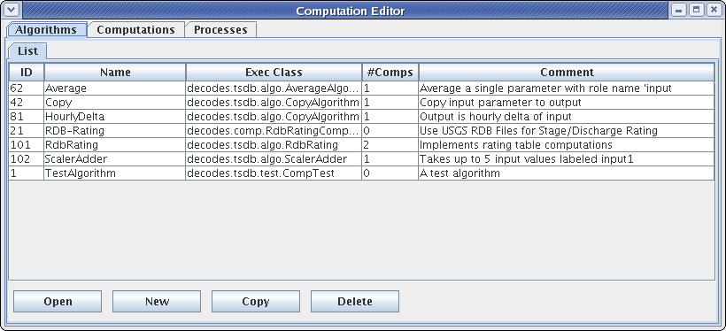
Figure 9: Computation Editor - Algorithms List Tab.

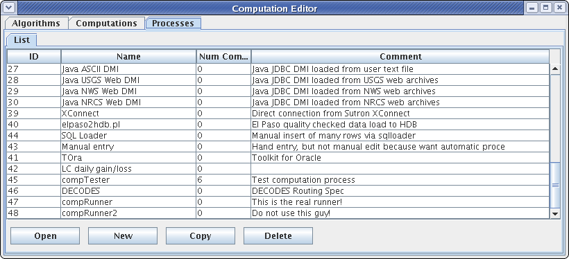
Figure 10: Computation Editor - Processes List Tab.

For the list of computations, you see a filter-area at the top of the screen (Figure 11). Since a database is likely to have hundreds or even thousands of computations, this allows you to quickly find the ones you are interested in. To use the filter, select any combination of filter-values and hit the ‘Refresh List’ button. The fields are …

• ‘Has Param at Site’ Select a site. Only computations with at least

  one parameter at that site are shown.

• ‘Has Param Code’ Type or select a parameter code. Only computations

  with a parameter with that code are shown.

• ‘Has Param Interval’ Select an interval. Only computations with a

  parameter with that interval are shown.

• ‘Process’ Select a computation process (a.k.a. loading application).

  Only computations assigned to that process are shown.

• ‘Algorithm’ Select an algorithm. Only computations using that

  algorithm are shown.

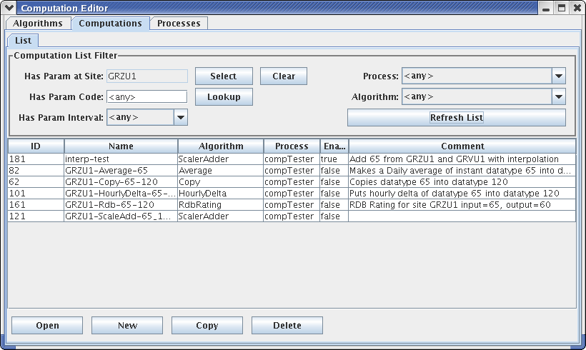
Figure 11: Computation Editor - Computation List Tab.

Action Buttons

Buttons along the bottom provide access to the detailed object information:

• Select an item in the list and press ‘Open’ to open an edit tab with the detailed information.

• Click ‘New’ to create a new object of the specified type.

• Select an item in the list and press ‘Copy’ to make a copy of an object with a different name and database ID.

• Select an item in the list and press ‘Delete’ to delete the item from the database.

Deleting Records that are ‘In Use’

In HDB, you will not be able to delete records that are ‘in-use’. This includes:

• Algorithms that are being used by one or more computations.

• Processes that have one or more computations assigned.

• Computations that have data in HDB.

Crisp First Line in Comment Areas

Note that the list tab shows only the first line of a possibly very long comment field. So please make the first line a good overall summary. Subsequent lines can provide more detail.

Sorting the Lists

Click on the column headers to sort the list by that column. This is useful for finding related records. For example, on the computation list tab, to find all computations using a particular algorithm, click on the Algorithm column header.

Algorithm Edit Tab

After pressing ‘Open’, ‘New’, or ‘Copy’ on the Algorithms List tab, you will see an open editor tab, as shown in Figure 12.

The main purpose of an algorithm record is to associate a name in database with a Java Class that will execute the algorithm. Creating the Java code for algorithms is covered in section 4.

It is important to keep in mind that the data in the Algorithm record must correspond to attributes in the Java code. For this reason, modifying algorithms is usually left to developers. See the separate manual CP-DevelopersGuide.

So why allow editing of algorithm meta-data here at all? One good reason is that there need not be a one-to-one relationship between Java classes and algorithm records. You could have several algorithm records that use the same Java class with different property settings, and even parameter definitions.

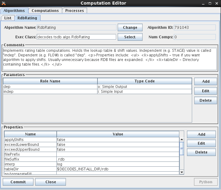
Figure 12: Computation Editor - Algorithm Editor Tab.

The fields in the algorithm edit tab include:

Algorithm Name: Every Algorithm has a unique descriptive name. Press the ‘Change’ button to the right of the field to change the name of an existing algorithm.

Algorithm ID: This field shows the unique database ID for this record.

Exec Class: This is the fully qualified Java Class name for this algorithm.

Num Comps: This is the number of computations that are currently making use of this algorithm.

Comment: Please type a complete description of your algorithm. Type a crisp opening line that will appear on the list tabs.

In the Parameters section you define the input and output time-series values to be used inside the algorithm. You define them by supplying a ‘role name’ and a type code.

To add a new parameter, press the ‘Add’ button to the right of the list. To edit an existing one, select it and then press ‘Edit’. In either case you see a dialog as shown in Figure 13.

Please refer back to Table 2‑2 for a list of parameter types. The Parameter dialog allows you to specify one of these types for this role.

Trick: The input parameter type need not agree with the type-code you defined when writing the algorithm Java code. For example, you could specify “idh” for hourly delta, when using the CopyAlgorithm. This would be an easy way to save a delta value to the database.

In the Properties area you specify non-time-series values. These are typically used to control features of the Java code. For example, the Java RdbRating code honors Boolean properties to allow it to do table looks that exceed the bounds of the table, and whether or not to apply the shifts found in the table. It has a String property specifying the directory where RDB files are to be found.

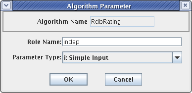
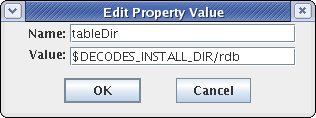
Figure 13: Algorithm Parameter and Property Dialogs.

Select Algorithm Executable Class

As of OpenDCS 6.1 RC15 there is a ‘Select’ button to the right of the Exec Class name. Prior to this you had to type the class name. Click the button and you are presented with a list of all known classes, as shown in the figure below:

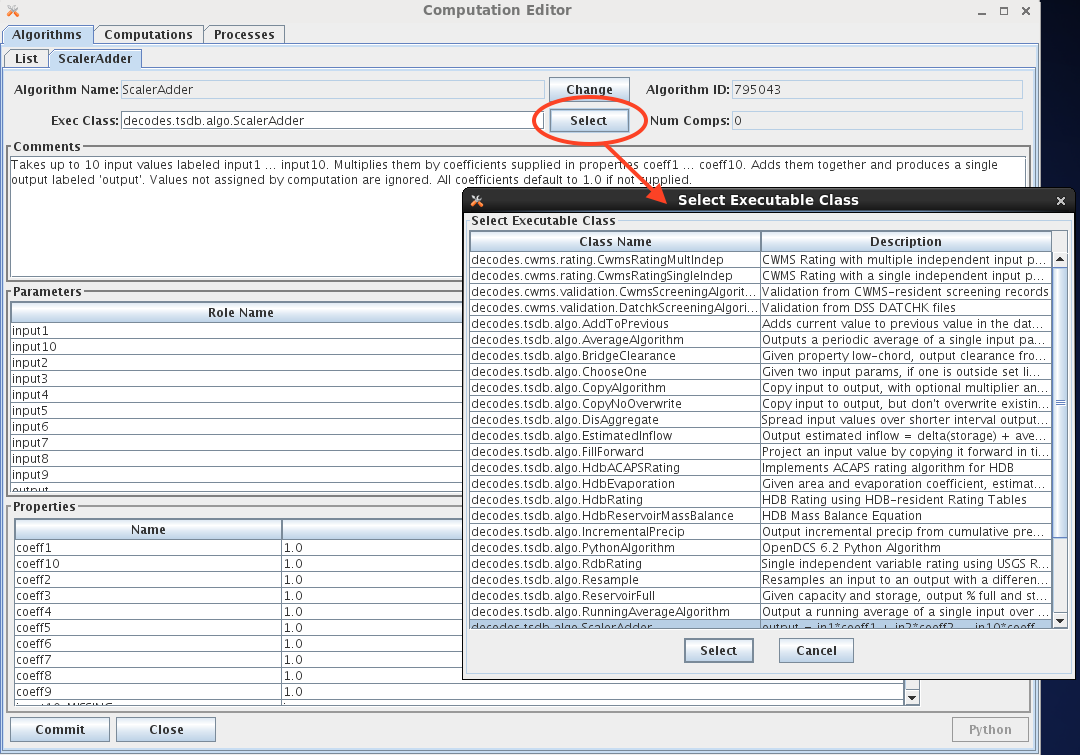
You can customize the list of class names that appear in this list by modifying one of two files:

• $DCSTOOL_HOME/doc/algorithms.txt (provided with the RC15 release)

• $DCSTOOL_USERDIR/algorithms.txt (for a multi-user installation)

The file has a single class per line. The first blank-delimited string on a line is the class name, the remainder of the line is a brief description.

If you have created your own classes, please annotate them in $DCSTOOL_USERDIR/algorithms.txt. This way, if you update in the future, your additions will not be lost. (The file in the doc subdirectory under the toolkit will be overwritten by an update!)

6-Hour Holdout Algorithm Example

Another example will illustrate the value in defining special algorithm records that modify the defaults defined in the Java code. See Figure 14.

The USGS Equation Algorithm takes one input, one output and four coefficients. It executes the equation:

output = A \* (B + input)^^C + D

Note the “type code” assigned to input. It is “id360” meaning that instead of operating on the input value directly, it will take the 6-hour delta (360 minutes).

Next we define A to be 2.0167. Why? Look at the EU (engineering units) definitions: The input is in ac-ft (Acre Feet). So we are looking at the change in storage in Acre Feet over 6 hours. But we want to output a FLOW in cfs (cubic feet per second), So …:

ac-ft/6Hours = cfs \* 2.0167

Thus we co-opted an existing algorithm to do a special purpose without writing any Java code!

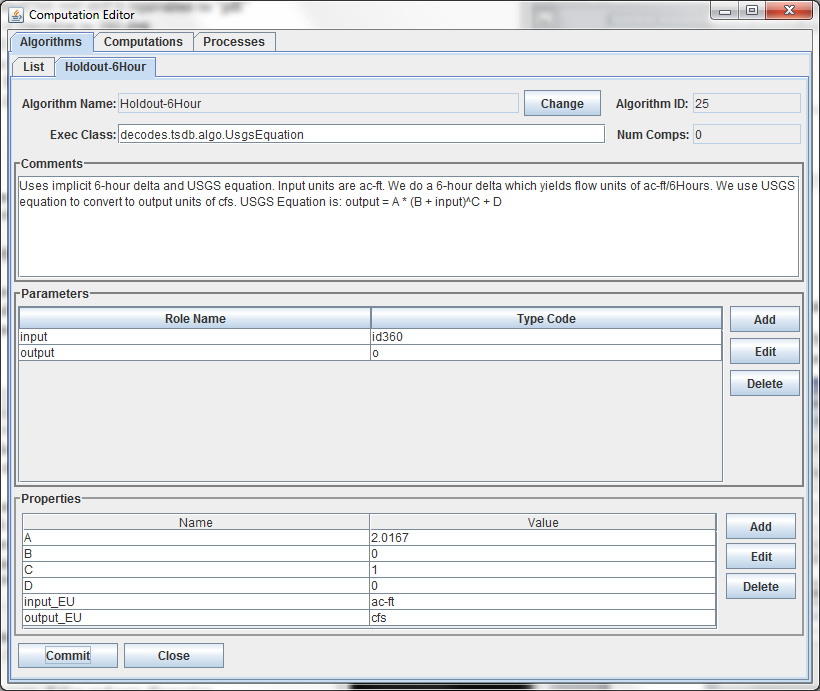
Figure 14: Algorithm record that customizes the UsgsEquation algorithm for a 6-hour holdout.

Computation Edit Tab

After pressing ‘Open’, ‘New’, or ‘Copy’ on the Computation List tab, you will see an open editor tab as shown in Figure 15 (for HDB) and Figure 16 (for CWMS).

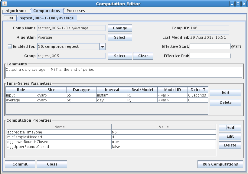
Figure 15: Computation Edit Tab for HDB.

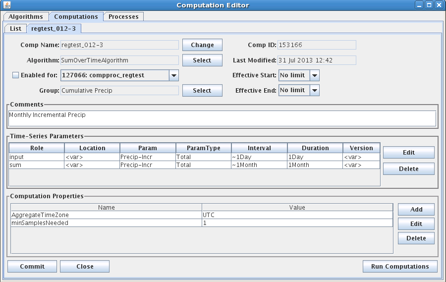
Figure 16: Computation Edit Tab for CWMS.

The fields in the computation edit tab include:

Comp Name: A unique symbolic name for this computation in the database. Press the ‘Change’ button to change a computation’s name.

Comp ID: The unique numeric ID assigned by the database when this computation is first saved. This is not editable.

Algorithm: Associates this computation with an algorithm in the database. Press the ‘Select’ button to select a different algorithm.

Last Modified: The date/time that this record was last modified in the database.

Effective Start: Input data before the specified time will not be processed by this computation. This value overrides any global “CpEffectiveStart” setting made in the decodes.properties file (see Error! Reference source not found.). You can specify the limit in three ways:

• No Limit (default setting) – no limit on lower end of date/time range

• Now minus some interval – (e.g. “now – 1 day”) This is evaluated when the computation is run. It allows you to specify that the computation is to process near real-time data only.

• Specified date/time – You specify a hard date/time value that is used.

  Effective End: Input data after the specified time will not be processed by this computation. You can specify the limit in four ways:

• No Limit (default setting) – no limit on upper end of date/time range

• Now – meaning do not process future data

• Now plus some interval – (e.g. now + 1 day) This allows the computation to process a limited amount of future data. For example if you are processing predicted stage value through the next 24 hours but never beyond that, you could enter “now + 25 hours”.

• Specified date/time – You specify a hard date/time value that is used.

  Enabled: Only computations that are enabled will be executed.

  Process: In order to be executed, you must assign the algorithm to a running process.

  Comment: Please type a complete description of your algorithm. The first line will appear in the description column in lists, so please make it a good overall summary. Subsequent lines can provide more detail.

The Edit/Delete buttons for computation parameters work much like they do in the Algorithm Tab. The computation parameter dialog is shown in Figure 17.

If you have deleted a parameter that is defined in the algorithm and want to add it back in later, just re-select the algorithm. It will bring in all undefined parameters again.

The Role Name area shows the selected algorithm role. In the rest of the fields you specify the location (site) data type, and other parameters necessary to point to a particular time series in your database.

Data Type can be typed directly, or you can press the ‘Lookup’ button a list of existing time series at the selected site. For inputs, you must select an existing data-type. For outputs, you can type a data-type that does not yet exist at that site and the system will create one.

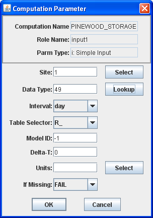
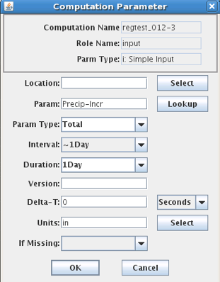
Figure 17: Computation Editor - Computation Parameter Dialog (HDB on left, CWMS on right).

Note also at the bottom of Figure 15, the button labeled ‘Run Computations’. Pressing this button will bring up the Interactive Run-Computations GUI described in chapter 9. The Run-Computations GUI will be linked to the Computation Edit screen such that changes made will be reflected in the run-computations without saving them first to the database.

Engineering Units

Note the “Units” field at the bottom of Figure 17. For some algorithms, it is important that you specify the correct units for the input and output. For example, if you are using an TAB Rating table that takes meters and outputs cubic meters per second, then you MUST specify these units in the parameter record. Otherwise the computation will be done using the default storage units for the underlying database, which in HDB are imperial units.

• When you specify units for an input param, the CP will convert the data into the correct units before performing the computation.

• When you specify units for an output param, the CP knows to do a conversion back to the correct storage-units for the parameter.

Options for handling Missing Data

For each input parameter, you can tell the computation processor what to do if a value is missing at a needed time. The possibilities are:

• FAIL – Don’t execute the algorithm at this time-slice.

• IGNORE – Execute the algorithm anyway. This is for algorithms with optional parameters like ScalerAdder that know how to proceed if an input parameter is not present.

• PREV – Execute the algorithm using the value just previous to this time slice.

• NEXT – Execute the algorithm using the value after this time slice.

• INTERP – Interpolate between the previous and next value.

• CLOSEST – Use either the PREV or NEXT value, whichever is closer in time.

In most cases, the default setting is made by the developer in the algorithm record and you should not change it.

Computation Properties

Note the properties settings at the bottom of Figure 15. Many algorithms take property settings to control various functions. See the individual section on each algorithm below for details.

Properties can be set in three places:

Computation Record overrides Algorithm Record overrides System defaults

Thus the computation record shown above is the final word on the property settings.

Running Computations Interactively

Before leaving the computation editor when you have created or modified a computation, it is recommended to press the ‘Run Computation’ button in the lower right corner. You will see a pop-up dialog as shown in Figure 18. Select the time-range over which to run the computation and press the Run button. The results are shown both graphically and in a table.

You can use this screen to execute computations over a historical time-period and then save the results to the database.

After you are satisfied that the computation is running properly, click the “Enabled” checkbox and assign it to the background computation processor “compproc”.

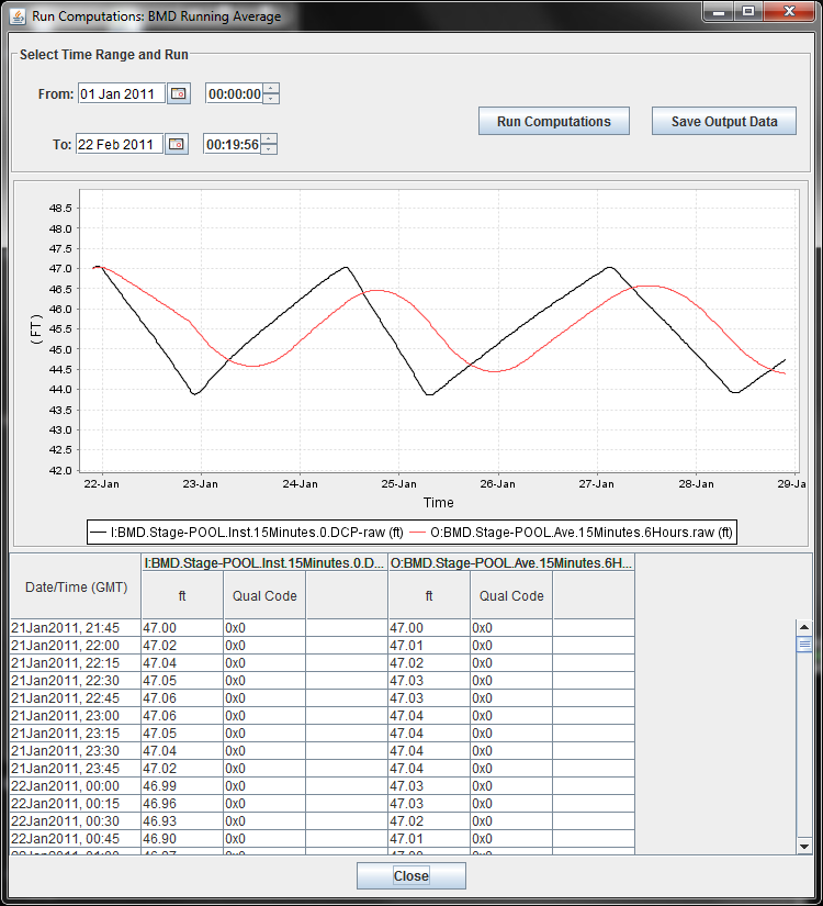
Figure 18: Run Computations Screen.

Process Edit Tab

After pressing ‘Open’, ‘New’, or ‘Copy’ on the Processes List tab, you will see an open editor tab as shown in Figure 19.

In HDB, a computation process is the same thing as a “LOADING APP”. It has a unique process name and ID (assigned by the database). It also has a free-form comment area.

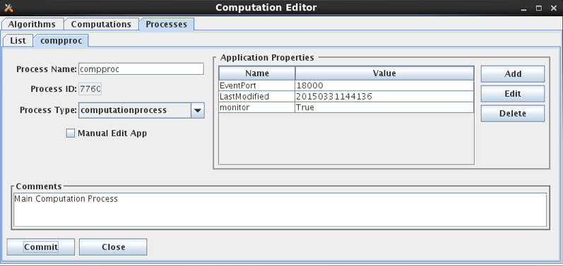
Figure 19: Computation Editor - Process Edit Tab.

New to OpenDCS 6.2 is the concept of a Process Type. Each process should be given a valid process type. You can create/edit the list of know process types with the OpenDCS Reference List Editor. Start it with the “rledit” command. Then, on the Enumerations Tab, select the “Application Type” Enumeration. You should see a list of known process types, as shown below.

Also on the process screen, notice two standard properties that are available to all daemon processes:

• monitor (true/false) – set to true to allow this process to be monitored in the new Process Status GUI.

• EventPort – For monitored processes, assign a unique event number to each. This enables the new Process Status GUI to connect and retrieve events from the process as they occur.

For OpenDCS 6.4 RC08 a new Computation Daemon property was added:

• reclaimTasklistSec – set to a number of seconds (default = 0). This is only used on Oracle Databases. If set to a positive number of seconds, then, when the tasklist is empty and this number of seconds has elapsed since the last attempt, the code will attempt to reclaim space allocated to the CP_COMP_TASKLIST table by issuing the following queries. The purpose is to shrink the allocated space back to something reasonable in case it has grown large.

ALTER TABLE cp_comp_tasklist ENABLE ROW MOVEMENT
ALTER TABLE cp_comp_tasklist SHRINK SPACE CASCADE
ALTER TABLE cp_comp_tasklist DISABLE ROW MOVEMENT

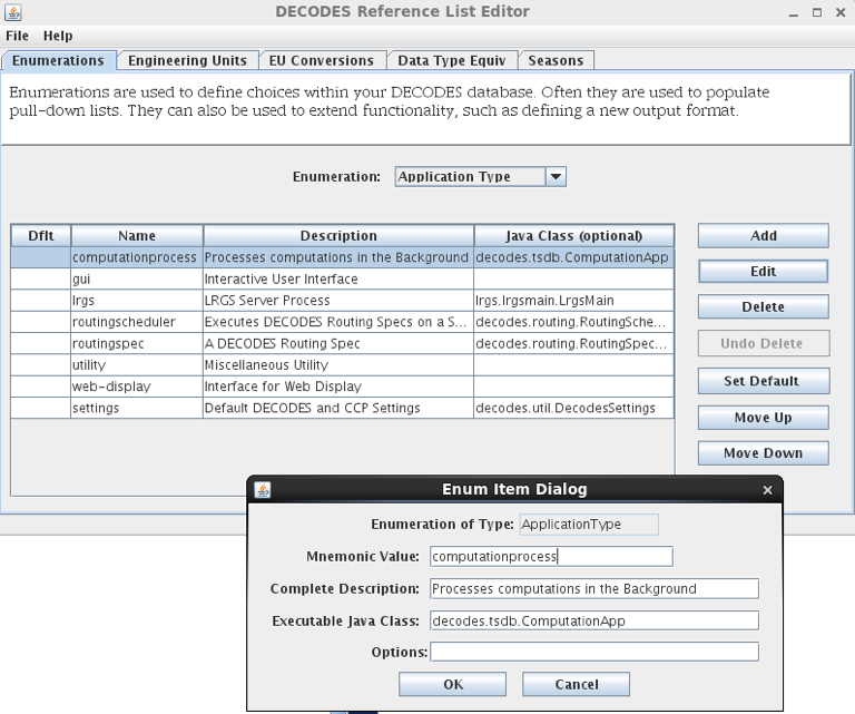
Figure 20: Application Type Enumeration

Time Series Groups and Computations

The above sections describe how to create and test computations that are assigned to specific time-series in the database. Do a quick estimate: How many water level parameters to you monitor? For each one, how many computations would you want to perform? For most organizations, this quickly becomes a very large number (hundreds or even thousands of computations).

This section will describe a way to define Time Series Groups, and then run your computations from the groups, rather than specific time-series. This will greatly reduce the number of computations you have to maintain.

Time Series Identifiers in HDB

An HDB Time Series is uniquely identified by:

• Site

• Data-Type (Site and Data-Type are sometimes combined into SDI)

• Interval: (instant, hour, day, month, year, or water year)

• Table-Selector: R_ (real) or M_ (modeled)

• Model-ID (modeled data only)

• Model-run-ID (modeled data only)

Some applications, such as the “outputts” (output time series) program described below, specify time series with a 4, 5, or 6 “path name”:

RUEWEACO.7.instant.R\_ Instantaneous real precip at site ‘RUEWEACO’
RUEWEACO.8.hour.M\_.1.1 Hourly modeled precip at the same site, model id and model run ID are both 1.

Time Series Identifiers in CWMS

CWMS uses a 6-part key:

Location.Param.ParamType.Interval.Duration.Version

For a complete discussion of CWMS Time Series Identifiers, see: U.S. Army Corps of Engineers (USACE) CWMS Standard Naming Conventions. WMIST (Water Management Implementation Support Team) Standard Naming Committee, March 2016.

As described in that document, Location, Param, and Version are often subdivided into multiple parts with a hyphen. The part up to the first hyphen is called the base part. After the first hyphen is called the sub part.

Examples:

• Location “Jefferson-Lower”.

  • Base Location is “Jefferson”. Sub Location is “Lower”.

• Location “Jefferson-Spillway-Tailwater”.

  • Base Location is “Jefferson”. Sub Location is “Spillway-Tailwater”.

• Location “L&D #24-Lock Chamber East”

  • Base Location is “L&D #24”. Sub Location is “Lock Chamber East”.

• Param “Temp-DewPoint-Air”

  • Base Param is “Temp”. Sub Param is “DewPoint-Air”.

• Param “Speed-Gust-Air”

  • Base Param is “Speed”, Sub Param is “Gust-Air”.

• Version “Rev-GOES”

  • Base Version is “Rev”. Sub Version is “GOES”.

Note that in the case of Location and Param, the distinction between base and sub part is formalized within the database (i.e. base and sub are stored in different table columns). In the Version string, this is not the case. The database stores it as a single 32-character string. For the purposes of CCP, however, it is treated the same as Location and Param.

What is a Time Series Group?

We have implemented a very flexible way of determine which time-series below to which groups. You can define a group in any of the following ways:

1. Select a set of specific time-series denoted by the full path name.

2. Specify one or more Locations: All time-series at the specified location(s) are members of the group.

3. Specify one or more Param designators. For example, a group called “Water-Levels” comprised of all time-series that have a param of 65 or 66.

4. Specify one or more Intervals. For example, all time series with interval of ‘instant’ or ‘Hour’.

5. Specify real or modeled data.

6. Specify one or more Model IDs.

7. A group may include all members of another group. For example you might have a “basin” group that includes several “river” groups.

8. A group may exclude all members of another group.

9. A group may be intersected with members of another group.

10. Any combination of the above.

Time Series Group Editor

Start the group editor in one of two ways:

• With the “groupedit” command line.

• Select “Groups” from the main Launcher bar.

Figure 21 shows the time series group editor. Like the other editors in computation processor and DECODES a list screen shows all the objects (groups) currently defined in the database. At the bottom you can open a group, create a new group, delete a group, or refresh the list.

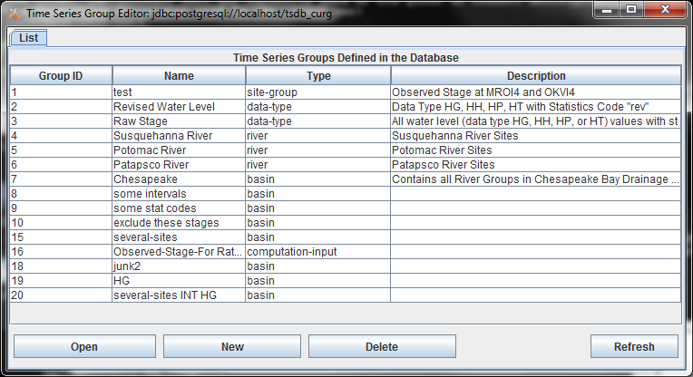
Figure 21: Time Series Group Editor List Screen

In the following descriptions, the HDB and CWMS versions of the GUI look slightly different because of the different components of a Time Series Identifier. The concepts are identical however.

Figure 22 shows a group that has been opened for editing. Following the figure, we will describe all the editing functions.

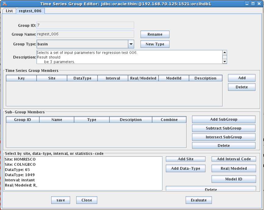
Figure 22: Time Series Group Editor - Open Group Screen.

The editor looks the same for HDB and CWMS except for the time series identifier components:

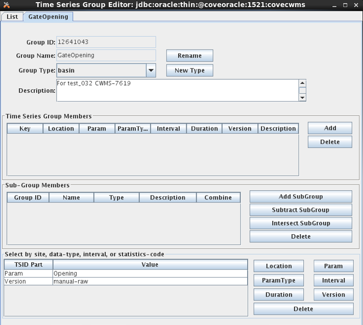
Figure 23: Time Series Group Editor for CWMS.

The button controls on this screen include:

Rename Press this button to rename the group. Every group in your database must have a unique name.

We recommend that you refrain from putting spaces in your group names. This is because names may be used on command-line utilities occasionally. Spaces in the name can cause command-parsing problems. So call your group “Raw-Stage” rather than “Raw Stage”.

New Type Each group is assigned a group type. You may define any number of group types. For example you might have a group type ‘River’ and then several groups that use this type for the rivers you maintain.

The Time Series Group Members Table is used to explicitly add time series to the group by specifying the complete path name.

Add Click this button to bring up a dialog of all time-series defined in your database. You may select one or more time-series from the list for inclusion in your group.

Delete Select a time-series in the list and click ‘Delete’ to remove a time-series from the group.

The Sub-Group Member Tableis used to combine other groups into this group that you are defining. There are three ways to combine:

Add SubGroup Add the members of another group into this group.

Subtract SubGroup Subtract the members of another group from this group. This is useful for special cases. E.g. you want all Revised Stage values EXCEPT the ones at a few specified sites.

Intersect SubGroup Intersect the members of a subgroup with this group. That is, only members contained in both groups will be included.

The Other-Criteria List is used to specify path-name parts for inclusion. You can filter by Site, Data-Type, Interval, Real/Modeled, or Model ID.

Evaluate the Group

Finally, notice the “Evaluate” button at the bottom right. Click this button to show you an expanded list of all existing time-series that would be considered members of this group as currently defined.

Filtering by Location, Param, and Version in CWMS

The Location, Param, and Version buttons in the lower right of the editor bring up special dialogs in CWMS in which you can specify full, base, or sub part.

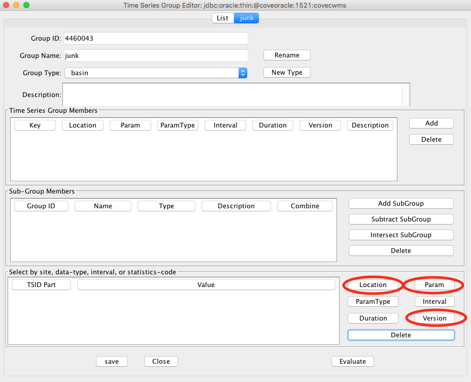
Figure 24: CWMS Special buttons for Location, Param, and Version.

The dialog for Location is shown below. The dialogs for Param and Version work the same way. The dialog shows you a list of all locations currently defined in the database. By clicking on the column headers, you can sort by base-part, sub-part, or the number of time series IDs that are currently defined at that location.

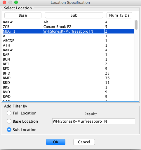
Figure 25: CWMS Group Editor Location Dialog.

At the bottom of the dialog are three radio buttons, which specify the type of filter you are adding:

• Full Location – Accept time series that match the selected full location (base and sub).

• Base Location – Accept time series that match the base location (any sub location is OK).

• Sub Location – Accept time series that match the sub location (any base location is OK).

If Sub Location is selected (or sub param or sub version in those dialogs), you may also include an asterisk ‘*’ as a wildcard. Do this by directly editing the Result field at the bottom of the dialog.

For example, if you edited the sub location field to be “Spillway*-Gate*”, it would match, for example, the following locations:

• ABC-Spillway1-Gate1

• XYZ-Spillway2-Gate5

Thus the asterisk will match any character except the hyphen.

Evaluating Time Series ID Components

You can specify any number of time series ID components using the buttons at the bottom of the editor. When you hit the Evaluate button, it will show you a list of time series which match the components you have specified.

You can specify multiple values for the same component, for example:

• Param: Stage

• Param: Flow

• Param: Stage-Bubbler

These are combined with a logical OR. Thus any time series that matches any of the 3 values will pass the filter.

If you specify values for different components, they are combined with a logical AND. Thus if you added to the above:

• Interval: 1Hour

• Duration: 0

Then of the time series with param Stage, Flow, or Stage-Bubbler, only those with interval 1Hour and duration 0 would pass the filter.

Using a Group in a Computation

To use a group in a computation, open the computation in the editor and select it from the list of groups. Then for each time series parameter, you specify a mask to be applied to each group member.

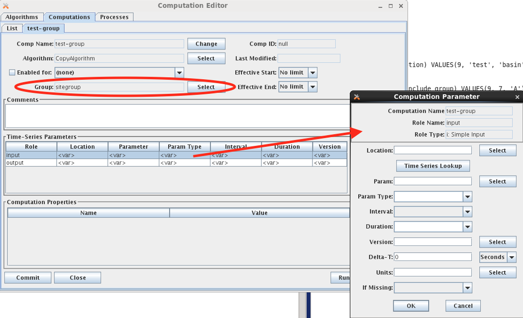
Figure 26: Using a Group in a Computation.

Note that the Computation Parameter dialog allows you to specify each time series identifier component individually. The values you specify will be substituted in the time series identifiers in the group.

Here’s how it works:

• The group is evaluated as described in the previous section. This results in a set of Time Series Identifiers (TSIDs) that are considered members of the group.

• When a computation uses that group, the set of TSIDs is applied to each input parameter as follows:

  • Replace the components in the TSID with the components specified in the Computation Parameter dialog.

  • This results in a different TSID. If this new TSID exists in the database, the computation can be executed. If not, it is skipped.

• Next the output parameters are resolved from the first input parameter in the same manner:

  • Replace the components in the input parameter TSID with the components specified in the dialog for the output. If the resulting TSID does not exist, it is created in the database.

Notice that specifying the computation parameter TSID components is not quite a filter. After applying the parameter mask, you could end up with a TSID which is not a group member. For example:

• A group called “Inst Stages” that contain any TSID with the param “Stage” and a duration of 0 (that is, an instantaneous value).

  • Suppose one of the TSIDs is “Hoover-Tailwater.Stage.Inst.15Minutes.0.raw”

• A computation called “Hourly Average Stage” which uses the group. The input parameter mask is wide open (i.e. it accepts all group members as-is.) The output parameter changes the interval and duration to 1Hour and the Param Type to Ave.

  • Input: Hoover-Tailwater.Stage.Inst.15Minutes.0.raw

  • Output: Hoover-Tailwater.Stage.Ave.1Hour.1Hour.raw

• A computation called “Hourly Flow” which uses the same group. The input parameter mask specifies interval=1Hour and duration=1Hour. Thus, this computation will use the TSIDs that are output from the first computation. Note that these TSIDs are not members of the group. The output changes the param to “Flow”.

  • Input: Hoover-Tailwater.Stage.Ave.1Hour.1Hour.raw

  • Output: Hoover-Tailwater.Flow.Ave.1Hour.1Hour.raw

• A computation called “Monthly Peak Flow”. It’s input parameter mask specifies param=Flow, interval=1Hour, and duration=1Hour. The output changes param=Flow-Peak, Interval=1Month

  • Input: Hoover-Tailwater.Flow.Ave.1Hour.1Hour.raw

  • Output: Hoover-Tailwater.Flow.Ave.1Month.1Hour.raw

Thus the entire chain operates from a single group. Except for the first computation in the chain, the input parameters are masked such that the computation is operating on TSIDs that are not members of the group.

As another example, suppose you have a group called “Reservoirs” which contains the Locations of all of your reservoirs. Then when the group is evaluated, it will contain all time series at those reservoirs, which may contain water levels, precipitation, temperatures, battery voltages, computed parameters, what-have-you. By specifying our input in the way described above, we filter the group so that our computation is only triggered by a subset of the group.

A Group Computation Example (HDB)

Figure 27 shows a computation that uses a group called “regtest_006”. Note the central area of the screen, which defines the Time-Series Parameters:

• Some of the path components are defined such as datatype, interval, and real/modeled.

• Some of the components are left variable.

When you define path components, these are substituted into the group members.

• For Inputs, this determines which time series will trigger the computation.

• For Outputs, this will determine the time series identifiers written to HDB.

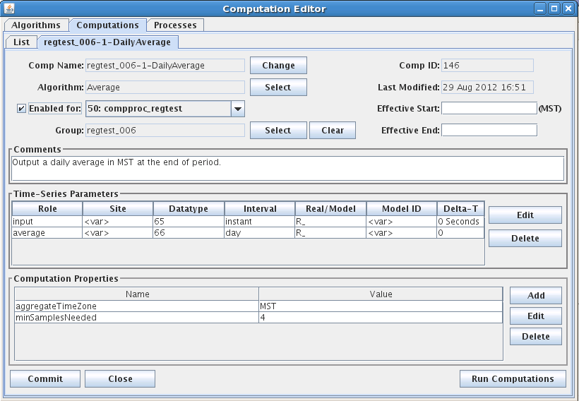
Figure 27: A Copy Computation with a Group Input

Computation Chains with Groups

As you can see, computations with groups are very flexible. Figure 28 provides an example for the Corps of Engineers CWMS database (but the concept is the same for HDB). Suppose you have a group called “Reservoirs” which contains a bunch of locations, including one called “BMD”. Now you use that group as the input for the three computations shown. Then you define the parameters as shown and see how the chain works!

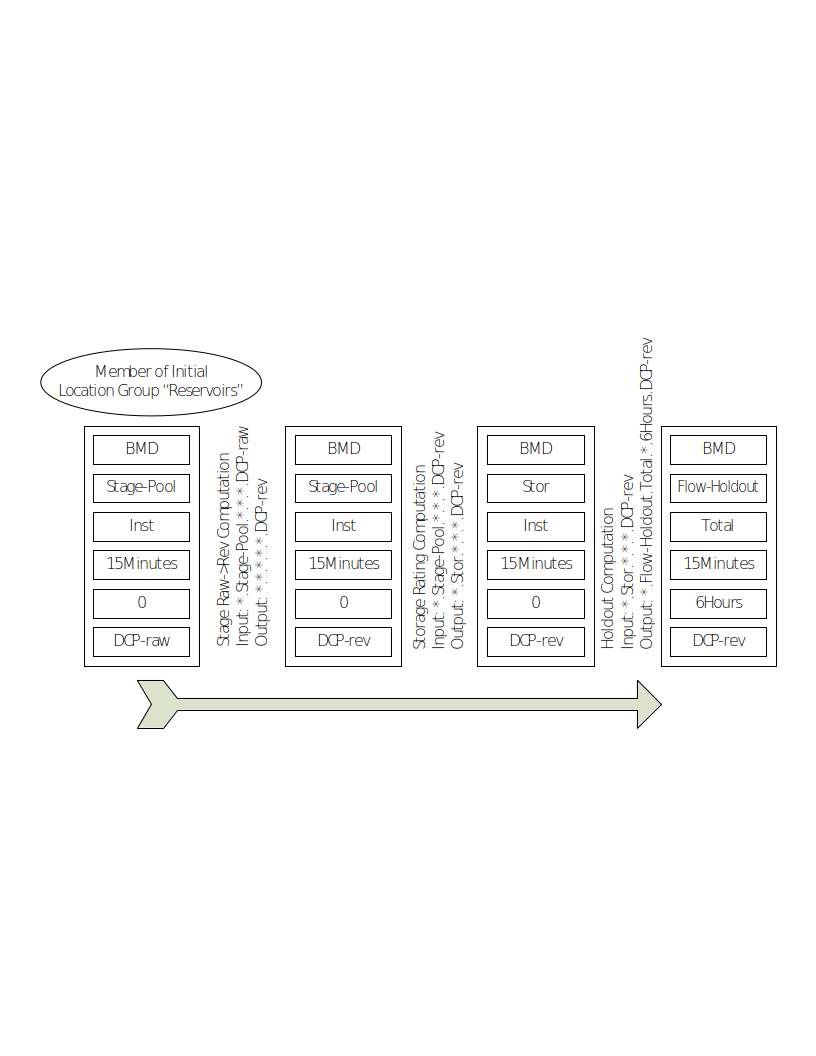
Figure 28: Chain of Computations with a Single Group.

CWMS Comp Param Substitution with Wildcards

This enhancement was added for OpenDCS 6.3 and only applies to CWMS.

A previous section describes how an asterisk can be used to denote a wildcard for Sub Location, Sub Param, or Sub Version in a group definition. A similar capability exists when applying parameter masks to these components.

The select buttons on the computation parameter screens bring up dialogs that are almost the same as the dialogs for groups. The location dialog is shown below.

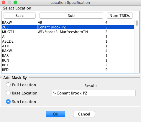
Figure 29: Computation Parameter Location Selection Dialog.

The only restriction is that an asterisk must be either at the beginning or end of the string, or must be bounded by hyphens. Recall that the mask is used to replace part of the TSID in the group members. The hyphen gives it the context it needs to do this.

Algorithms Provided in the Computation Processor

The first section below describes properties that are common to different algorithm classes (time-slice, aggregating, running-aggregate). Following this, a subsection is provided for each algorithm supplied with the CP distribution.

Common Properties to Algorithms

The following tables describe properties used by the computation infrastructure and are thus common to all algorithms or all algorithms of a given class. They can be set in algorithm records (to apply to all computations using an algorithm) or computation records (to apply to a specific computation).

Property names are NOT case sensitive.

Properties Common to All Algorithms:

Name	Java Type	Description
debugLevel	long	This property overrides the “-d” argument used when compproc is started. Thus you can increase debug level for a particular algorithm (by defining the property in the algorithm record) or for a particular computation. 0=no debug, 1=more debug, 2=even more, 3=most verbose.
TIMEROUND	long	Default=60 (seconds). Time series values with time-tags within this many seconds are considered to be at the same time-slice.
interpDeltas	Boolean	Default = false. When computing an automatic delta, if one of the bounding values is missing and this is set to true, then the CP can interpolate the missing value in order to compute the delta. This is subject to the ‘maxInterpIntervals’ property.
maxInterpIntervals	long	Default = 10. See ‘interpDeltas’ above. When CP interpolates in order to compute an automatic delta. It will not interpolate if more than this many contiguous values are missing.
aggregateTimeZone	String	Default is set in decodes.properties. This can be set on an algorithm or computation to override the default. It must be one of Java’s valid time-zone identifiers. This is also used inside debug messages in the log when displaying a time-series value.
rolen ame_MISSING	String	See section 3.4.2. Normally this is set in the computation parameter dialog. You can set it in your algorithms to establish a default.

Properties for Aggregating Algorithms:

Name	Java Type	Description
aggregateTimeZone	String	(default set in decodes.properties)
aggLowerBoundClosed	Boolean	(default=true) True means to include the lower bound of the aggregate period in the calculation.
aggUpperBoundClosed	Boolean	(default=false) True means to include the upper bound of the aggregate period in the calculation.
aggregateTimeOffset	String	(default = no offset, i.e. aggregate period starts at beginning of even interval). Syntax is: N period … Where N is a positive integer and period is one of year, month, day, hour, minute, second. You can have multiple specifications like: “1 day 4 hours”
noAggregateFill	Boolean	(default=false) If set to True, then CP will not iterate time slices for aggregate computations. This accommodates algorithms that want to perform the aggregate in the database.
maxMissingValuesForFill	Integer	See section 2.5.6. This property provides an upper limit to the number of values that the computation processor will automatically fill missing values.
maxMissingTimeForFill	Integer	This is a number of seconds. See section 2.5.6. This property provides an upper limit to the amount of time that the computation processor will automatically fill missing values.

Properties for Running Aggregate Algorithms:

Name	Java Type	Description
aggPeriodInterval	String	(No default, required). For running aggregates, the aggregate period interval is set independently from the interval of the output parameter. Syntax is dbInterval or dbInterval * count where dbInterval is a valid interval string in the underlying database and count is an integer.
aggregateTimeZone	String	(default set in decodes.properties)
aggLowerBoundClosed	Boolean	(default=true) True means to include the lower bound of the aggregate period in the calculation.
aggUpperBoundClosed	Boolean	(default=false) True means to include the upper bound of the aggregate period in the calculation.
noAggregateFill	Boolean	(default=false) If set to True, then CP will not iterate time slices for aggregate computations. This accommodates algorithms that want to perform the aggregate in the database.

AddToPrevious

Type: Time Slice

Input Parameters:

Name	Java Type	Type Code
Input	double	i

Output Parameter:

output : double precision

Properties:

Name	Java Type	Default
minSamplesNeeded	long	1

Description:

Adds the current value to the previous value in the database and outputs the sum. Works on any time-series, any interval. This algorithm does assume that you are calling it with a series of contiguous values, like you would get out of a DCP message.

Average

Type: Aggregating – period defined by output parameter “average”.

Input Parameters:

Name	Java Type	Type Code
Input	double	i

Output Parameter:

average : double precision

Properties:

Name	Java Type	Default
minSamplesNeeded	long	1
outputFutureData	Boolean	False
aggPeriodInterval	String	(no default – required)
aggregateTimeZone	String	(default set in decodes.properties)
aggLowerBoundClosed	Boolean	False
aggUpperBoundClosed	Boolean	True
aggregateTimeOffset	String	No offset. I.e. aggregate period starts at beginning of even interval
negativeReplacement	double	No default. If set, and the average value to be output is negative, then replace it with this value.

Description:

This is a general purpose averaging algorithm. The aggregating period will be determined by the “interval” value that you assign to the output variable “average”. Thus it is useful for producing a wide variety of averages.

Your computation record should set an appropriate value for the “minSamplesNeeded” property, depending on the output period and the interval of the input parameter.

This algorithm fail and not produce an output if the required number of points is not present in the aggregating period.

It will attempt to delete its output if any of the input points was flagged as being deleted. This handles the case where there used to be an average, but some of the input points are deleted and there is no longer the required minimum.

In version 5.2 the aggregateTimeOffset period has been added. This allows you to compute averages other than midnight to midnight.

Bridge Clearance

Type: Time-Slice

Input Parameters:

Name	Java Type	Type Code
waterLevel	double	i

Output Parameter:

clearance : double precision

Properties:

Name	Java Type	Default
lowChord	double	1

Description:

Computes bridge clearance by subtracting waterlevel from constant ‘low chord’.

Make sure that the waterlevel and low chord are consistent. If one is a stage above arbitrary datum, then they both must be. Likewise, if one is an elevation above sea level, the other must be also.

Choose One

Type: Time-Slice

Input Parameters:

Name	Java Type	Type Code
input1	double	i
input2	Double	i

Output Parameter:

output : double precision

Properties:

Name	Java Type	Default
upperLimit	double	999999999999.9
lowerLimit	Double	-999999999999.9
chooseHigher	Boolean	True
input1LowThreshold	Double	(none)

Description:

Useful in situations where you have redundant sensors: Given two inputs, output the best one:

• If only one is present at the time-slice, output it.

• If one is outside the specified upper or lower limit (see properties) output the other.

• If both are present and within limits, then it chooses based on other properties:

• If the input1LowThreshold property is supplied, then

  Output input1 if its value is above the low threshold

  Otherwise output input2.

• Otherwise (input1LowThreshold not supplied), if chooseHigher==true

  (the default) then output the higher of the two, otherwise the lower of the two.

Copy

Type: Time-Slice

Input Parameters:

Name	Java Type	Type Code
Input	double	i

Output Parameter:

output : double precision

Properties:

Name	Java Type	Default
mult	double	1.0
offset	Double	0.0

Description:

Copies its input to its output with an optional multiplier and offset.

You can use this algorithm to save delta values to the database as follows:

• In the Computation Editor, make a copy of the algorithm record called “HourlyDelta”.

• In this record change the input type code to “idh”.

• Create a computation record to use the new algorithm.

Likewise, you can use this algorithm for any type of delta (daily, monthly, etc.) by changing the input type code appropriately.

This algorithm will delete its output if its input is deleted.

Copy No Overwrite

This algorithm is the same as the plain Copy algorithm with the following exceptions:

• It will not overwrite the output if a value already exists at the same time.

• It does not support the “mult” property.

Dis-Aggregate

Type: Time-Slice

Input Parameters:

Name	Java Type	Type Code
input	double	i

Output Parameter:

output : double precision

Properties:

Name	Java Type	Default
method	String	“fill”

Description:

This algorithm ‘dis-aggregates’ by spreading out the input values to the outputs in various ways (fill or split). The interval of the input should always be equal to, or longer than, the output. The output value is filled over the time-period of the inputs.

For example: Input is daily, and the output is hourly. Then 24 output values are written covering the period of each input.

The algorithm takes one property called ‘method’. This determines how the output values are assigned:

• fill (default) - Each output is the same as the input covering the period.

• split - Divide the input equally between the outputs for the period.

Recall from the definitions in section 2.5.4, that a time-slice algorithm iterates over all available input parameters. That is indeed what the dis-aggregate algorithm does, although it produces more than one output per input. Thus this is a time-slice algorithm.

Incremental Precip

Type: Aggregating

Input Parameters:

Name	Java Type	Type Code
cumulativePrecip	double	I

Output Parameter:

incrementalPrecip: double precision

Properties:

Name	Java Type	Default
aggLowerBoundClosed	Boolean	True
aggUpperBoundClosed	Boolean	True
allowNegative	Boolean	False

Description:

Compute Incremental Precip from Cumulative Precip over a specified period.

Period determined by the interval of the output parameter, specified in computation record.

If property allowNegative is set to true, then negative cumulative Precip inputs will be accepted. The default is to ignore negative inputs.

Resample

Type: Aggregate – period defined by output parameter “output”.

Input Parameters:

Name	Java Type	Type Code
input	double	i

Output Parameter:

output : double precision

Properties:

Name	Java Type	D efault	Description
method	String	“interp”	Determines how to set outputs for which there is no input in the period. For example, going from DAY to HOUR values. If set to “interp” then each hour will be an interpolation between the day values. You can also set the property to “fill”, meaning that each hour will be set to the previous daily value.

Description:

Resample an input to an output with a different interval. Output must not be instant (irregular). Input may be irregular or any interval greater than or less than the output.

Note, The Subsample algorithm is more efficient when converting a short interval to a long interval (e.g. output a daily value by selecting the midnight hourly value).

Reservoir Full

Type: Time Slice

Input Parameters:

Name	Java Type	Type Code
storage	double	i

Output Parameter:

percentFull : double precision

storageRemaining : double precision

Properties:

Name	Java Type	Default
capacity	double	1

Description:

Given reservoir storage (output of rating computation), and a property ‘capacity’, output the percent full and storage remaining.

Running Average

Type: Running-Aggregate – period defined by output parameter “average”.

Input Parameters:

Name	Java Type	Type Code
input	double	i

Output Parameter:

average : double precision

Properties:

Name	Java Type	Default
minSamplesNeeded	long	1
outputFutureData	Boolean	False
aggPeriodInterval	String	(no default – required)
aggregateTimeZone	String	(default set in decodes.properties)
aggLowerBoundClosed	Boolean	False
aggUpperBoundClosed	Boolean	True

Description:

This outputs a running average at the same interval as the input parameter.

The aggregate period is set by the “aggPeriodInterval” property, which must be a valid interval-string in the underlying database. For example:

• In HDB, you could use hour, day, month, year, or wateryear.

• In CWMS, you could use 6Hours, 1Day, etc.

You can also add a multiplier. For example “hour*12” would mean twelve hours.

The “minSamplesNeeded” property works just like it does in the simple Average Algorithm: If less than this many ‘input’ values are present in an aggregate period, no ‘average’ will be produced.

Note that this algorithm can produce future data. For example, suppose ‘input’ is at an interval of 1Hour, minSamplesNeeded is set to 12, and aggPeriodInterval is set to “1Day”. Then, when a 9AM value appears in real time, it will compute averages from 9AM through 9PM. After that, there will be less than 12 samples.

To prevent future data from ever being computed, set the ‘outputFutureData’ property to false.

CentralRunningAverage

Type: Running Aggregate

Introduced in Version: 6.2 RC05

To make this algorithm visible after installing an update, run:

cd $DCSTOOL_HOME

bin/compimport imports/comp-standard/CentralRunningAverageAlgorithm.xml

USACE added a separate algorithm called CentralRunningAverage. It is identical to Running Average (described above) except that the outputs are time tagged at the center of the period. The time tag is determined to second-resolution by splitting the different between the beginning of one period and the next.

Caution: If the aggregate time zone is one that honors daylight time the aggregate periods may not be of equal length (example: daily running average computed every hour for time zone EST5EDT). For the days when daylight time changes, the “day” being averaged will be either 23 or 25 hours. Thus the center of period will be either 11.5 or 12.5 hours after the start of period.

An alternate way to accomplish this with more control would be to use Running Average (described in previous section) and put a Delta-T on the output parameter.

ScalerAdder

Type: Time-Slice

Input Parameters:

Name	Java Type	Type Code
input1	double	i
input2	double	i
input3	double	i
input4	double	i
input5	double	i
Input6	double	i
Input7	double	i
Input8	double	i
Input9	double	i
Input10	double	i

Output Parameter:

output : double precision

Properties:

Name	Java Type	Default
coeff1	double	1.0
coeff2	double	1.0
coeff3	double	1.0
coeff4	double	1.0
coeff5	double	1.0
coeff6	double	1.0
coeff7	double	1.0
coeff8	double	1.0
coeff9	double	1.0
coeff10	double	1.0
input1_MISSING	String	“ignore”
input2_MISSING	String	“ignore”
input3_MISSING	String	“ignore”
input4_MISSING	String	“ignore”
input5_MISSING	String	“ignore”
input6_MISSING	String	“ignore”
input7_MISSING	String	“ignore”
input8_MISSING	String	“ignore”
input9_MISSING	String	“ignore”
input10_MISSING	String	“ignore”

Description:

This algorithm can take up to 10 inputs, multiply them by supplied coefficients and add them together. In summary:

output = (input1 * coeff1)

• (input2 * coeff2)

• (input3 * coeff3)

• (input4 * coeff4)

• (input5 * coeff5)

• (input6 * coeff6)

• (input7 * coeff7)

• (input8 * coeff8)

• (input9 * coeff9)

• (input10 * coeff10)

The algorithm checks to make sure each value is present before multiplying by it’s coefficient and adding it to the output.

Note the default setting of “ignore” on the MISSING properties. This makes the algorithm useful for adding from 1 to 10 points. Your computation record should override these values to “fail” for required inputs.

Subsample

Type: Aggregating

Input Parameters:

Name	Java Type	Type Code
inputShortInterval	double	I

Output Parameter:

outputLongInterval: double precision

Properties:

Name	Java Type	Default
aggLowerBoundClosed	Boolean	True
aggUpperBoundClosed	Boolean	False

Description:

Subsamples the input parameter by the interval of the output parameter. For example, you could produce an hourly value by subsampling 15-minute input values.

Sum Over Time

Type: Aggregating

Input Parameters:

Name	Java Type	Type Code
Input	double	I

Output Parameter:

sum: double precision

Properties:

Name	Java Type	Default
aggLowerBoundClosed	Boolean	False
aggUpperBoundClosed	Boolean	True
minSamplesNeeded	Integer	1

Description:

Sum the input values over the period of the output.

Rating Calculations with USGS RDB Files

Type: Time-Slice

Input Parameters:

Name	Java Type	Type Code
Indep	double	i

Output Parameter:

dep : double precision

Properties:

Name	Java Type	Default
exceedLowerBound	boolean	False
exceedUpperBound	boolean	False
tableDir	String	$DECODES_INSTALL_DIR/rdb

Description:

This algorithm uses the USGS RDB rating-table files to do a stage-to-flow (or elevation-to-volume) conversion.

It looks for a file in the specified “tableDir” directory with a name of the form:

UsgsSiteNum.rdb

You can download these files for any USGS site from the following URL:

http://nwis.waterdata.usgs.gov/nwisweb/data/exsa_rat/filename

… wherefilename is constructed as above.

The two ‘exceed’ properties tell the algorithm how to handle the situation where the input value is below the lowest table value or above the highest. The default behavior is to fail to produce an output. By setting these properties to ‘true’, you can cause it to extend the interpolation of the two lowest or highest values.

Rating with simple ASCII Table Files

Type: Time-Slice

Input Parameters:

Name	Java Type	Type Code
indep	double	i

Output Parameter:

dep : double precision

Properties:

Name	Java Type	Default
exceedLowerBound	boolean	False
exceedUpperBound	boolean	False
tableDir	String	$DECODES_INSTALL_DIR/tab-files
tableName	String	(empty string)
tableNameSuffix	String	.tab

Description:

This algorithm uses the rating table files to do a stage-to-flow (or elevation-to-volume) conversion.

It looks for a file in the specified “tableDir” directory with a name of the form:

SiteName + suffix

Or, you can completely specify the “tableName” property directly.

The two ‘exceed’ properties tell the algorithm how to handle the situation where the input value is below the lowest table value or above the highest. The default behavior is to fail to produce an output. By setting these properties to ‘true’, you can cause it to extend the interpolation of the two lowest or highest values.

USGS Equation

Type: Time-Slice

Input Parameters:

Name	Java Type	Type Code
input	double	i

Output Parameter:

output : double precision

Properties:

Name	Java Type	Default
A	double	1.0
B	double	0.0
C	double	1.0
D	double	0.0

Description:

Implements the USGS Equation:

output = A \* (B + input)^C + D

where A, B, C, and D are provided as properties.

Fill Forward

Type: Time-Slice

Introduced in Version: 5.3

Input Parameters:

Name	Java Type	Type Code
input	double	i (simple input)

Output Parameter:

output : double precision

Properties:

Name	Java Type	Def ault	Description
numIntervals	Integer	4	Maximum number of output intervals to fill forward. Set to 0 for no limit.

Description:

This algorithm is used to project an input value by copying it forward in time for the specified number of intervals. This is used for certain modeling programs.

For example, suppose the following parameters:

• Input: OKVI4.Stage.Inst.1Hour.0.rev

• Output: OKVI4.Stage.Inst.1Hour.0.fill

• NumIntervals: 4

Now suppose the 08:00 input value of 5.23 arrives. This algorithm will set the following output values: (08:00 5.23), (09:00 5.23), (10:00 5.23), and (11:00 5.23).

The algorithm will fill-forward until one of the following:

• the specified maximum number of intervals is reached

• the next input is reached

• the current time is reached.

The input and output interval may be different. Filling will start on the first output time after or equal to the input time. It also honors the aggregateTimeZone and aggregateTimeOffset properties:

Example:

• Input OKVI4.Stage.Inst.1Hour.0.rev

• Output: OKVI4.Stage.Inst.~1Day.0.fill

• NumIntervals: 4

• AggregateTimeZone: EST5EDT

• AggregateTimeOffset: 5 hours

Now suppose the Jan 5 08:00 EST input value of 5.23 arrives. This algorithm will set the following output values: (Jan 6 05:00 EST 5.23), (Jan 7 05:00 EST 5.23), (Jan 8 05:00 EST 5.23), and (Jan 9 05:00 EST 5.23).

An enhancement was added in 6.5 RC04 to allow filling to either the current time or the next input value (whichever is earlier). To do this:

• Set the numIntervals property to 0 (zero).

• Set the maxMissingValuesForFill property to a number large enough to cover the period you want filled. Example: if the values have interval 1Hour and you need to fill 4 days, then set to at least 4 * 24 = 96.

• Set the maxMissingTimeForFill property to a number of seconds large enough to cover the period you want filled. Example: if fill 4 days, then set to at least 4 * 86400 = 345600.

Expression Parser Algorithm

Type: Time-Slice

Introduced in Version: 6.1 RC11

To make this algorithm visible after installing an update, run:

cd $DCSTOOL_HOME
bin/compimport imports/comp-standard/ExpressionParserAlgorithm.xml

Input Parameters:

Name	Java Type	Type Code
in1	double	i (simple input)
in2	double	i (simple input)
in3	double	i (simple input)
in4	double	i (simple input)
in5	double	i (simple input)

Output Parameter:

out1 : double precision

out2 : double precision

Properties:

Name	Java Type	Def ault	Description
pre_*	String	(none)	Lines of script to execute before time slices.
ex_*	String	(none)	Lines of script to execute for each time slice.
post_*	String	(none)	Lines of script to execute after each time slice.

Description:

This algorithm allows you to write your own scripts using mathematical expressions. The scripts are stored in properties. There are 3 separate scripts:

• All properties with names beginning with “pre_” are sorted into a script and executed once before time slices. This script is typically used for looking up meta data to be used during the time slices.

• All properties with names beginning with “ex_” are sorted into a script and executed for each time slice. Assignments made to the output variables, out1 and out2, cause data to be written to the database.

• All properties with names beginning with “post_” are sorted into a script and executed once after all of the time slices.

The expression parser is based on JEP (Java Expression Parser). A discussion of JEP syntax and capabilities can be found here:

http://www.cin.ufpe.br/~gfsv/gfsv/workspace/jep-2.4.1-ext-1.1.1-gpl/doc/html/

In addition to the standard syntax and all the standard mathematical constants and functions, the following custom functions have also been added:

lookupMeta(location, param)	FUTURE IMPLEMENTATION. This function looks up meta data for a given location.
cond(cond, expr)	If the cond expression evaluates to true, then execute the second argument expr and return its value. Typically this is an assignment, like this: cond(in2 < 915.0, tabname=in1.site + “,”) else(tabname = in2.site)
else(expr)	This would normally be on the line following the cond() function. If the previous cond function resulted in false (such that its expression was not evaluated) then the expression in the else(expr) statement here will be evaluated.
exit()	Typically included in some kind of conditional expression like if, cond, or else. This function returns 0. It also sets a flag causing the execution of the script to stop.
goto(expr)	‘expr’ should result in a string that matches one of your property name statement labels. The function itself returns zero. After execution the next statement label is set.
debug3(expr) debug2(expr) debug1(expr) info(expr) warning(expr)	These statements cause messages to be written to the computation processor log. Each message will be prefixed with the date/time and name of the computation.
onError(expr)	‘expr’ should result in a string that matches one of your property name statement labels. This is usually used near the beginning of a script. If any subsequent statement results in an error, then execution jumps to the named label.
rating(specId, in1,in2…inN)	The first argument is the string rating spec ID. Subsequent arguments are the independent input values for the rating. The rating spec determines the number of input variables allowed.

datchk(inputName)	The argument is the variable name (e.g. “in1” in double quotes). The function performs whatever screenings are defined for the named parameter at the current time slice. It returns the resulting quality flags. These are usually assigned to the flags associated with the variable, as in: in1.flags = datchk(“in1”)
screening(inputName)	This performs screening according to screening records in the CWMS database.
isQuestionable(parm.flags)	Returns true if the passed flags-value indicates that the value is marked as QUESTIONABLE. This is used to check the result of screening. Example, the following will perform a datchk screening and set set the flags on the input parameter. Then, if the result of the screening is not REJECTED, the value and flags are set. in1.flags = datchk(“in1”, in1) cond(isQuestionable(in1.flags), warning(”…”))
isRejected(parm.flags)	Returns true if the passed flags-value indicates that the value is marked as REJECTED. This is used to check the result of screening. Example, the following will perform a datchk screening and set set the flags on the input parameter. Then, if the result of the screening is not REJECTED, the value and flags are set. in1.flags = datchk(“in1”) cond(isRejected(in1.flags), exit()) out1 = in1 out1.flags = in1.flags

The following constants can be used in your expressions:

Name	** Type**	Description
in1	Number	The value of the in1 parameter in this timeslice.
in1.Location	String	Location of the time series associated with in1
in1.Param	String	The ‘param’ part of the time series ID associated with in1
in1.ParamType	String	ParamType part of the TS ID associated with in1
in1.Interval	String	Interval part of the TS ID associated with in1
in1.Duration	String	Duration part of the TS ID associated with in1
in1.Version	String	Version part of the TS ID associated with in1
in1.ParamType	String	ParamType part of the TS ID associated with in1
in1.ParamType	String	ParamType part of the TS ID associated with in1
in1.baseloc	String	The base location of the TS ID associated with in1
in1.subloc	String	The sub location of the TS ID associated with in1
in1.baseparam	String	The base param of the TS ID associated with in1
in1.subparam	String	The sub param of the TS ID associated with in1
in1.baseversion	String	The portion of the version string up to the first hyphen, of the entire string if no hyphen is present
in1.subversion	String	The portion of the version string after the first hyphen, or unassigned if no hyphen is present
in1.flags	Number	A long integer representation of the data quality and other flags associated with the input value. These are used by the screening and datchk methods.
in2…in5	as above	For all input params you can reference the value or the parts of the time series ID as described above for in1.
out1 out2	Number	Initially, out1 and out2 have no value. Your script at some point should make an assignment to one or both of them. After an assignment is made, the value may be used in other expressions.
out1.t sid-part out2.t sid-part	String	The time series ID parts may be referenced for both output parameters in the same way as described above.
out1. flags out2. flags	Number	A long integer representation of the data quality and other flags associated with the output value. These are used by the screening and datchk methods.

WARNING! Care should be taken to ensure that you do not write a script that results in an endless loop. Since looping is possible in a variety of contexts, the algorithm code has no way of detecting all the ways that an endless loop can happen.

As implied in the table above, at some point your time slice or post script should make assignments to one or both of the output parameters. After executing a script (e.g. in a timeslice), the code checks to see if an assignment was made, and if so, a time-series value is written to the database.

A quirk of the JEP parser is apparent when combining strings and numbers, which will be common in the expressions in the logging functions. Use JEP’s str() function to convert numbers to strings before combining with other strings:

info("in1 = " + str(in1) + ", in2=" + str(in2))

Example of Using Expression Parser for Conditional Rating

The figure below shows an example of using the Expression Parser algorithm for a conditional rating.

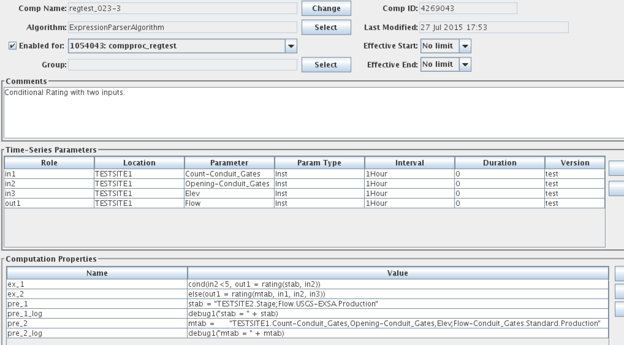
Figure 30: Expression Parser used for Conditional Rating

Note the three inputs defined and the single output. Now see the two properties ex_1 and ex_2. these form the following script:

cond(in2 < 5, out1 = rating(stab, in2))
else(out1 = rating(mtab, in1, in2, in3))

Thus if the value at a given time for in2 (TESTSITE1.Opening-Conduit_Gates.Inst.1Hour.0.test) is less than 5, then the single-variable rating defined by stab is used. Otherwise (in2 >=5) the multi-variable rating defined by mtab is used.

See how stab and mtab are defined in the ‘pre’ script.

Division Algorithm

Type: Time-Slice

Introduced in Version: 6.2 RC05

To make this algorithm visible after installing an update, run:

cd $DCSTOOL_HOME

bin/compimport imports/comp-standard/Division.xml

Input Parameters:

Name	Java Type	Type Code
input1	double	i (simple input)
input2	double	i (simple input)

Output Parameter:

output : double precision

Properties:

Name	Java Type	Def ault	Description
a	Double	1.0	Multiplier for input1
b	Double	0.0	Adder for input1
c	Double	1.0	Multiplier for input2
d	Double	0.0	Adder for input2

Description:

Implement the equation:

output = ((a * input1) + b) / ((c * input2) + d)

No output is produced if the right side of the division operator evaluates to 0.

Weighted Water Temperature

Type: Time-Slice

Introduced in Version: 6.2 RC05

To make this algorithm visible after installing an update, run:

cd $DCSTOOL_HOME

bin/compimport imports/comp-standard/WeightedWaterTemperature.xml

Input Parameters:

Name	Java Type	Type Code
input1	double	i (simple input)
input2	double	i (simple input)
input3	double	i (simple input)
input4	double	i (simple input)

Output Parameter:

output : double precision

Properties:

(none)

Description:

Implement the equation:

output = ((input1 / input2) \* input3) + (1 – (input1 / input2) \*
input4)

No output is produced if the input2 is less than or equal to zero.

FlowResIn – Compute Reservoir Inflow at LRP

Type: Time-Slice

Introduced in Version: 6.2 RC05

To make this algorithm visible after installing an update, run:

cd $DCSTOOL_HOME
bin/compimport imports/comp-standard/FlowResIn.xml

Input Parameters:

Name	Java Type	Type Code
ResOut	double	i (simple input)
Dstore	double	id (Delta with implicit period)

Output Parameter:

ResIn : double precision

Properties:

averageSamples (default=1)

Description:

Computes estimated reservoir inflow using measured outflow and change in storage.

The Dstore interval must be one of:

• 15minutes

• 1hour

• 1day

• ~1day

The algorithm converts the change in reservoir storage (DStore) from acre-ft per interval (one of the allowed intervals) and adds it to the measured ResOut (which should be in cfs), and then assigns the result to ResIn.

An alternate, more flexible way of computing reservoir inflow using Python Algorithm is described in section 6.6.

Multiplication Algorithm

Type: Time-Slice

Introduced in Version: 6.2 RC05

To make this algorithm visible after installing an update, run:

cd $DCSTOOL_HOME
bin/compimport imports/comp-standard/Multiplication.xml

Input Parameters:

Name	Java Type	Type Code
input1	double	i (simple input)
input2	double	i (simple input)

Output Parameter:

output : double precision

Properties:

Name	Java Type	Def ault	Description
a	Double	1.0	Multiplier for input1
b	Double	0.0	Adder for input1
c	Double	1.0	Multiplier for input2
d	Double	0.0	Adder for input2

Description:

Implement the equation:

output = ((a \* input1) + b) \* ((c \* input2) + d)

Stat (Statistics) Algorithm

Type: Aggregating

Introduced in Version: 6.2 RC09

To make this algorithm visible after installing an update, run:

cd $DCSTOOL_HOME
bin/compimport imports/comp-standard/Stat.xml

Time Series Parameters:

Role Name	Type	Description
input	input	The input time series.
ave	output	The average of the inputs over the period.
min	output	The minimum of the inputs over the period.
max	output	The maximum of the inputs over the period.
med	output	The median of the inputs over the period.
stddev	output	The standard deviation of the inputs over the period.

You may leave the statistics undefined if desired. For example, if you only want min, max, and average, leave median and stddev undefined. If this is a group-based computation, you should also set the ‘enabled’ properties listed below to prevent them from being automatically defined.

The interval of the time series assigned to the ‘ave’ output is used to determine the aggregate period. It is up to you to make sure that the time series assigned to the outputs each has the same interval. If ‘ave’ is undefined, you may use the built-in ‘aggPeriodInterval’ property to define the aggregate period.

The output units are set to the input units.

Properties:

Property Name	Java Type	D efault	Description
aggPeriodInterval	String	(none)	If defined, this will be used to define the aggregate period. Normally this is taken from the Interval of the time series assigned to the ‘average’ output.
aveEnabled	boolean	true	If false, no average output is produced.
minEnabled	boolean	true	If false, no minimum output is produced.
maxEnabled	boolean	true	If false, no maximum output is produced.
medEnabled	boolean	true	If false, no median output is produced.
deviationEnabled	boolean	true	If false, no standard_deviation output is produced.
minSamplesNeeded	long int	1	If fewer than this many inputs are present in the period, then no output is produced.

PeriodToDate Algorithm

Type: Aggregating

Introduced in Version: 6.4 RC04

To make this algorithm visible after installing an update, run:

cd $DCSTOOL_HOME

bin/compimport imports/comp-standard/PeriodToDate.xml

Time Series Parameters:

Role Name	Type	Description
input	input	The input time series.
periodToDate	output	The output period-to-date values go here. Must have same interval as input.
determineAggPeriod	output	Used only to determine the aggregate period. See below.

This algorithm behaves like a time-slice algorithm in that it outputs an value for each input value, and that the input and output (periodToDate) parameters must have the same interval.

A second output parameter, ‘determineAggPeriod’, is used only to determine the aggregating period. That is, when the to-date values are to be reset. No values are ever written to this time series, but it must exist in the database.

Example: To do a daily year-to-date value, set input to the time series with the daily values. Set periodToDate to the time series that will hold the output year-to-date values. Set determineAggPeriod to any yearly time series in the database.

Properties:

Property Name	Java Type	D efault	Description
goodQualityOnly	boolean	false	If set to true, then only good quality input values will contribute to the output periodToDate tally.

GroupAdder Algorithm

Type: Time Slice

Introduced in Version: 6.6 RC01

To make this algorithm visible after installing an update, run:

cd $DCSTOOL_HOME

bin/compimport imports/comp-standard/GroupAdder.xml

Time Series Parameters:

Role Name	Type	Description
mask	input	Applied to members of the group to determine the time series to sum. The Missing Action assigned to this parameter determines how to handle values that are missing at a given time slice (see below).
sum	output	The sum of the masked group members.
count	output	optional output set to the number of inputs processed
average	output	optional output set to the average of inputs

This algorithm provides a way to sum members of a group. It is a good alternative to ScalarAdder and BigAdder in cases where the coefficient is always 1.

It is designed to run efficiently as a timed computation (see section 2.7). You can have the computation run periodically at a time when the input values are expected to be present. It can be run in the normal fashion, as a triggered computation, but be aware that the computation will then run when each individual input arrives, which may be asynchronously.

The group is expanded to a set of time series identifiers. The mask is then applied, which may modify the time series identifiers. Data is fetched for each time series and then summed. The output sum is written to the database.

The Missing Action assigned to the ‘mask’ parameter determines how the algorithm handles the case where one or more of the time series does not have a value at a given time slice. Section 2.5.6 describes the possible values.

Python Algorithms

Beginning with OpenDCS 6.2 RC04 you have the ability to write algorithms that use Python scripts to execute your computations.

Creating a New Python Algorithm

In the Computation Editor, on the Algorithm tab, click New. Then click the Select button to the right of Exec Class. Select decodes.tsdb.algo.PythonAlgorithm from the list.

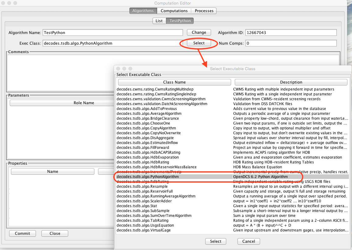
As a demonstration, we will create a Python algorithm that does a validation of a Stage input “rawstage” to produce “revstage”. It then does a rating on “revstage” to produce “flow”. Since the algorithm can be triggered by either rawstage or revstage, both are defined as inputs. Flow is defined as an output.

• Use Case: A user uses a GUI to modify a revstage value.

Use the Add button to the right of the Parameters window to create the time series parameters for the algorithm:

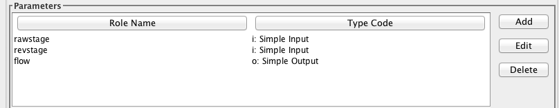
Now, notice that when PythonAlgorithm is selected, the Python button in the lower right of the screen is now enabled. Press it now.

You can write three different scripts:

• A script executed before each group of time-slices. This is useful for initializing variables (like tallies and counters), as well as opening any external resources the algorithm needs.

• A script executed at each time slice

• A script executed after each group of time-slices

What defines a ‘group of time-slices’? This depends on the Algorithm Type. There are three types:

• TIME_SLICE (the simplest type): CCP will collect all the new input values. It will execute the Before script once. It will execute the Time Slice script for each discrete time in the data. It will execute the After script once when finished.

• AGGREGATING: For example, for a Daily Average, the Before script is executed for each Day seen in the input data. Use it to set the tally and count to zero. The Time Slice script is executed for each value in the day. Use it to add to the tally and increment the count. The After script is executed after all the values for a given day are processed. Use it to output the daily average.

• RUNNING_AGGREGATE: Like AGGREGATING, but the aggregate period is specified in a property rather than the interval of the output.

Our example is a simple TIME_SLICE algorithm.

Now in the ‘Before Time Slices’ tab we create a simple script that sets a CWMS Rating Spec ID. The script is shown below.

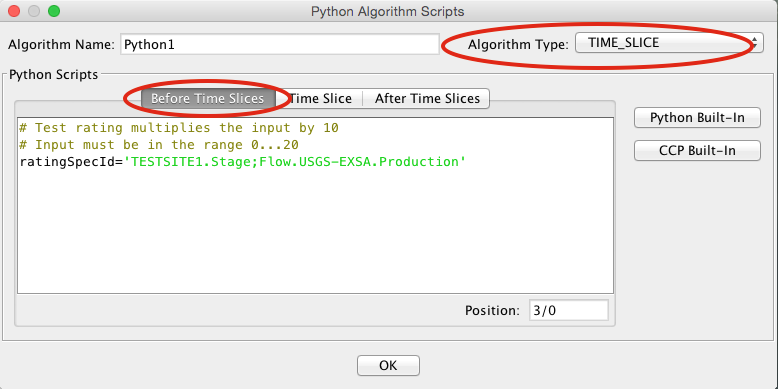
Now click the Time Slice tab. The bulk of the work is done here.

As an aid while typing your script, you can click the CCP Built-In button. This gives you an annotated list of built-in functions for interfacing with CCP and the CWMS database. You can select a function from the dialog to have it inserted into your code.

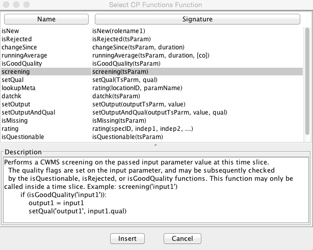
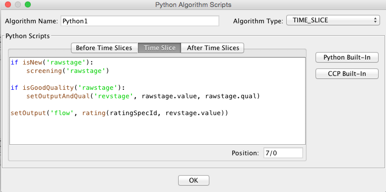
Here is the script text. We will go through it line by line.

if isNew('rawstage'):
   screening('rawstage')
if isGoodQuality('rawstage'):
   setOutputAndQual('revstage', rawstage.value, rawstage.qual)
setOutput('flow', rating(ratingSpecId, revstage.value))

The first two lines of the script are:

if isNew('rawstage'):
   screening('rawstage')

The isNew() function will return true if the named parameter is either a triggering value or a derived value in this time slice:

• A triggering value comes from a tasklist entry. It is what caused this computation to run.

• A derived value is one that was just computed in this computation and is flagged for output to the database.

Why do the isNew() check? Suppose this computation was triggered by someone using a GUI to modify a revstage value. In such a case there is no need to redo the screening on rawstage.

The screening() function looks for a CWMS Screening record for the named parameter. If found, it is applied to the current timeslice value and the quality flags set appropriately.

The next two lines are:

if isGoodQuality('rawstage'):
   setOutputAndQual('revstage', rawstage.value, rawstage.qual)

The isGoodQuality() function will return true if the results of the screening are OK. That is, the value is present, and it is not flagged as Questionable or Rejected. We only want good values copied to the revstage parameter.

The setOutputAndQual() function copies the passed value and quality to the named parameter. Notice how the value and quality of rawstage are referenced.

The final block of code is:

setOutput('flow', rating(ratingSpecId, revstage.value))

Notice call to the rating function embedded in the call to setOutput():

rating(ratingSpecId, revstage.value)

We pass it the ratingSpecId that was computed in the Before Time Slices script. We then pass it the current value for revstage. The rating() function can take multiple independent variables. If it fails for any reason it will not produce an output and the call to setOutput will do nothing.

When we ran this computation with a batch of test values, the output was as follows. We set the screening such that the top two and lower two values are Rejected. The next two on either side are Questionable. The Rating was constructed to output a value ten times the input for easy verification.

UTC	rawstage	revstage	flow
01/01/2012 00:00:00	0.00 SR
01/01/2012 01:00:00	1.00 SR
01/01/2012 02:00:00	2.00 SQ
01/01/2012 03:00:00	3.00 SQ
01/01/2012 04:00:00	4.00 S	4.00 S	40.00
01/01/2012 05:00:00	5.00 S	5.00 S	50.00
01/01/2012 06:00:00	6.00 S	6.00 S	60.00
01/01/2012 07:00:00	7.00 S	7.00 S	70.00
01/01/2012 08:00:00	8.00 S	8.00 S	80.00
01/01/2012 09:00:00	9.00 S	9.00 S	90.00
01/01/2012 10:00:00	10.00 S	10.00 S	100.00
01/01/2012 11:00:00	11.00 S	11.00 S	110.00
01/01/2012 12:00:00	12.00 S	12.00 S	120.00
01/01/2012 13:00:00	13.00 S	13.00 S	130.00
01/01/2012 14:00:00	14.00 S	14.00 S	140.00
01/01/2012 15:00:00	15.00 S	15.00 S	150.00
01/01/2012 16:00:00	16.00 S	16.00 S	160.00
01/01/2012 17:00:00	17.00 S	17.00 S	170.00
01/01/2012 18:00:00	18.00 S	18.00 S	180.00
01/01/2012 19:00:00	19.00 S	19.00 S	190.00
01/01/2012 20:00:00	20.00 SQ
01/01/2012 21:00:00	21.00 SQ
01/01/2012 22:00:00	22.00 SQ
01/01/2012 23:00:00	23.00 SR
01/02/2012 00:00:00	24.00 SR

Accessing the Time Slice Time Value

A special variable named “tsbt” is available to your python code. This holds the double-precision “tick” value of the time slice base time. You can use any of the functions in the Python “time” package to manipulate the value as date/time components or strings.

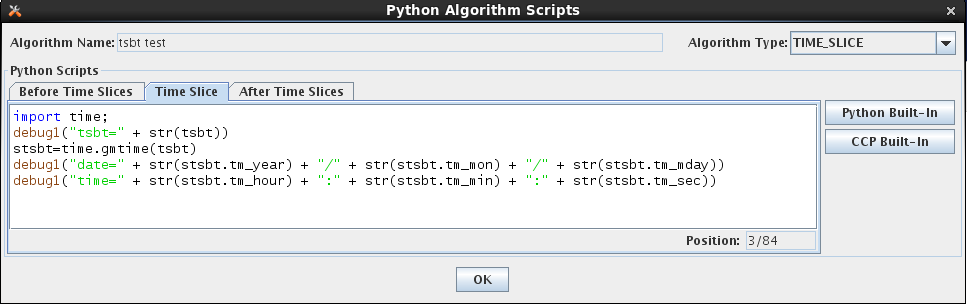
Creating a Computation that Uses the Algorithm

You create computations for Python algorithms in the same way you do for any other algorithm. The figure below shows a computation assigned to our new “Python1” algorithm. Concrete time series identifiers are assigned to each of the “roles” defined in the algorithm.

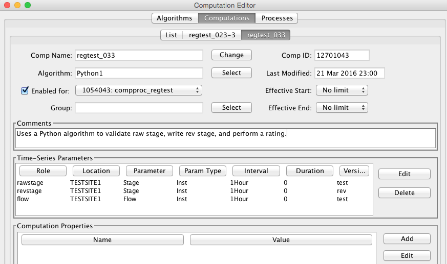
Time Series Parameters in the Python Scripts

Two variables are always available to your scripts:

loading_application_id This is set to the ID (surrogate key) of the application used to connect to the database when the computation processor (or compedit if you’re running the computation interactively) started up.

computation_id This is set to the ID (surrogate key) of the computation record in the database.

As you noticed in the above example, you can access time-series variables within your script. Use the dot-notation to specify what you want to access in the time series:

rolename.value The value of the time series at the current time-slice (may only be used in the Time Slice script.)

rolename.qual The quality flag value of the time series at the current time-slice (may only be used in the Time Slice script.)

rolename.tsid The String time series identifier, or TSID.

rolename.tskey The surrogate key for this TSID in the database. For CWMS, this is the numeric ts_code. For HDB this is the key in to the CP_TS_ID table (i.e. CP_TS_ID.TS_ID).

rolename.interval The Interval portion of the TSID.

CWMS-Specific Time Series Meta Data:

rolename.location The location portion of the TSID

rolename.baselocation The base location of the TSID or the entire location if there is no hyphen separater in the string.

rolename.sublocation The sub location of the TSID, or empty if there is no hyphen.

rolename.param The Param portion of the TSID

rolename.baseparam The base param of the TSID, or the entire param if there is no hyphen

rolename.subparam The sub param of the TSID, or empty if there is no hyphen.

rolename.paramtype The ParamType portion of the TSID (e.g. Inst, Total)

rolename.duration The Duration portion of the TSID

rolename.version The Version portion of the TSID

rolename.baseversion The base version of the TSID, or the entire version if there is no hyphen

rolename.subversion The sub version of the TSID, or empty if there is no hyphen

HDB-Specific Time Series Meta Data:

rolename.sdi The Site Datatype ID of the time series (in HDB, this is distinct from tskey).

rolename.site The DECODES preferred site name for the location of the TSID.

rolename.tableselector This will be R_ for real data or M_ for modeled.

rolename.modelId If this time series is modeled data, this will be the model ID.

Also notice that several of the built-in CCP functions take a role name as an argument. See how the isNew() function is called:

if isNew(‘rawstage’):

Conditional Rating Example

For another example we will do a conditional rating. We define a new Python Algorithm with the following parameters:

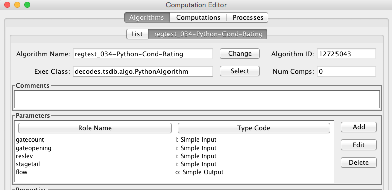
We have a reservoir with gates. The first three parameters are a count of the gates, the gate opening in feet, and the reservoir level. The forth parameter is the stage for the reservoir tail. The final output parameter flow is rated as follows:

• If stagetail is less than 5.0 we using a single-variable rating that depends only on stagetail.

• If stagetail is greaterthan or equal to 5.0 we use a 3-variable rating with independent parameters count, opening, and reslev.

There are two CWMS-resident rating tables. In the Before Time Slices script we construct the CWMS Rating Spec IDs:

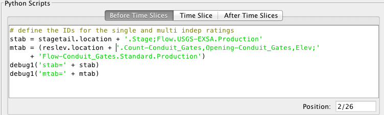
Notice how the locations are taken from the parameters to build the complete Spec IDs. The debug1() function will print the names of the tables to the log.

The Time Slice script is now very simple:

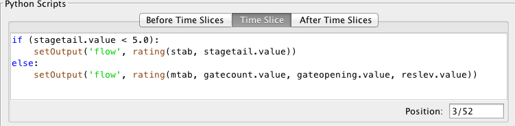
Reservoir Estimated Inflow

For a more complex example we will computed estimated inflow for a reservoir that measures only pool elevation and tail-water stage. The computation is illustrated as follows:

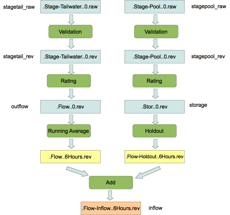
In the past, each of the green rounded boxes would be a separate computation. We will implement the entire chain in a single Python algorithm. To start, we define a new Python Algorithm as follows. Notice that we define time series parameters for each of the labels to the left and right of the figure above. Also, the yellow boxes labeled “.Flow..6Hours.rev” and “.Flow-Holdout..5Hours.rev” will exist only inside the Python script. They will not be written to time series in the database.

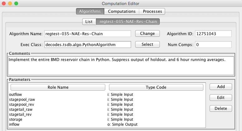
We will be doing two ratings using RDB and simple TAB files. In the Before script we define the file names, again using the location from the time series parameters:

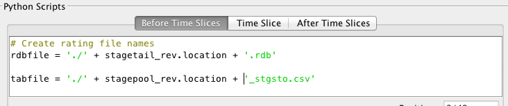
We assume the files will be in the current directory (where compproc is running). That’s why we use the “./” prefix, meaning current directory. You could also use a hard coded path name.

The Time Series script is as follows:

# Copy no-overwrite from stagetail raw to rev

if isNew('stagetail_raw') and not isGoodQuality('stagetail_rev'):

setOutputAndQual('stagetail_rev', stagetail_raw.value,
stagetail_raw.qual)

# Rating from stagetail rev to outflow

if isNew('stagetail_rev'):

try:

setOutput('outflow', rdbrating(rdbfile, stagetail_rev.value))

except NoValueException as e:

warning(e.toString())

# 6 hour running average of outflow is not saved to a time series

if isNew('outflow'):

ave6hrOutflow = runningAverage('outflow', '6Hours', '(]')

# 2nd part of chain: Stage Pool

if isNew('stagepool_raw') and not isGoodQuality('stagepool_rev'):

setOutputAndQual('stagepool_rev', stagepool_raw.value,
stagepool_raw.qual)

# Rating from stagepool to storage

if isNew('stagepool_rev'):

try:

setOutput('storage', tabrating(tabfile, stagepool_rev.value))

except NoValueException as e:

warning(e.toString())

# Holdout is a 6hr delta storage converted from acre-ft to cfs (not
saved)

if isNew('storage'):

try:

holdout = changeSince('storage', '6Hours') \* 2.0167

# Finally, the inflow is outflow + holdout.

setOutput('inflow', ave6hrOutflow + holdout)

except NoValueException as e:

warning('Error in changeSince: ' + e.toString())

Note how each block begins with ‘isNew()’ containing the name of the parameter that would trigger that block of code. This is so we only do the amount of work needed: Imagine if the computation were triggered by a GUI edit of stagepool_rev: Only the 2^nd half of the script would be run, starting with the tabrating for storage.

Also notice the exception handling in the final block of code: The rating, averaging, and changeSince functions can raise a NoValueException if they are unable to produce an output. It’s important to catch this to prevent the computation from terminating without saving its output.

XML Import/Export Utilities

Computational Meta-Data can be exported to, and imported from, XML files. This section describes the XML format and the import/export utilities.

XML Format for Computation Meta-Data

Figure 31 contains an example meta-data file. The file contains:

• One Computation Process Record (a.k.a. Loading Application) called “compTester”.

• Two Algorithm Records called “Copy” and “RdbRating”.

• Two Computation Records called “GRZU1-Copy-65-120” and “GRZU1-Rdb-65-60”.

The example illustrates all aspects of the XML format

<?xml version="1.0" standalone="yes"?>

<CompMetaData>

<LoadingApplication name="compTester">

<Comment>Test computation process.

Modified comment</Comment>

</LoadingApplication>

<Algorithm name="Copy">

<Comment>

Copy input parameter to output. Delete output if input was deleted.

</Comment>

<ExecClass>decodes.tsdb.algo.CopyAlgorithm</ExecClass>

<AlgoParmroleName="input">

<ParmType>i</ParmType>

</AlgoParm>

<AlgoParmroleName="output">

<ParmType>o</ParmType>

</AlgoParm>

</Algorithm>

<Algorithm name="RdbRating">

<Comment>

Implements rating table computations. Holds the lookup table & shift

values. Independent (e.g. STAGE) value is called "indep".

Dependent (e.g. FLOW) is called "dep". <p>Properties

include: <ul> <li>applyShifts - true if you want algorithm to

apply shifts. Usually unnecessary because RDB files are expanded.

</li> <li>tableType - default="RDB". Also supports

"SimpleTable". </li> <li>tableDir - Directory

containing table files.</li> </ul>

</Comment>

<ExecClass>decodes.tsdb.algo.RdbRating</ExecClass>

<AlgoProperty name=”exceedUpperBound”>false</AlgoProperty>

<AlgoProperty name=”applyShifts”>false</AlgoProperty>

<AlgoProperty name=”exceedLowerBound”>false</AlgoProperty>

<AlgoProperty name=”tableDir”>$DECODES_INSTALL_DIR/rdb</AlgoProperty>

<AlgoParmroleName=”dep”>

<ParmType>o</ParmType>

</AlgoParm>

<AlgoParmroleName=”indep”>

<ParmType>i</ParmType>

</AlgoParm>

</Algorithm>

<Computation name=”GRZU1-Copy-65-120”>

<Comment>Copies datatype 65 into datatype 120.</Comment>

<Enabled>false</Enabled>

<CompProcName>compTester</CompProcName>

<AlgorithmName>Copy</AlgorithmName>

<LastModified>2006-09-26 11:33:47 EDT</LastModified>

<CompParmroleName=”input”>

<SiteDataType>

<SiteNameNameType=”nwshb5”>GRZU1</SiteName>

<SiteNameNameType=”usgs”>09234500</SiteName>

<DataType Standard=”HDB”>65</DataType>

</SiteDataType>

<Interval>instant</Interval>

<TableSelector>R_</TableSelector>

<DeltaT>0</DeltaT>

</CompParm>

<CompParmroleName=”output”>

<SiteDataType>

<SiteNameNameType=”nwshb5”>GRZU1</SiteName>

<SiteNameNameType=”usgs”>09234500</SiteName>

<DataType Standard=”HDB”>120</DataType>

</SiteDataType>

<Interval>instant</Interval>

<TableSelector>R_</TableSelector>

<DeltaT>0</DeltaT>

</CompParm>

</Computation>

<Computation name=”GRZU1-Rdb-65-60”>

<Comment>RDB Rating for site GRZU1 input=65, output=60</Comment>

<Enabled>true</Enabled>

<CompProcName>compTester</CompProcName>

<AlgorithmName>RdbRating</AlgorithmName>

<LastModified>2006-09-26 15:04:22 EDT</LastModified>

<CompProperty name=”tableDir”>.</CompProperty>

<CompParmroleName=”dep”>

<SiteDataType>

<SiteNameNameType=”nwshb5”>GRZU1</SiteName>

<SiteNameNameType=”usgs”>09234500</SiteName>

<DataType Standard=”HDB”>60</DataType>

</SiteDataType>

<Interval>instant</Interval>

<TableSelector>R_</TableSelector>

<DeltaT>0</DeltaT>

</CompParm>

<CompParmroleName=”indep”>

<SiteDataType>

<SiteNameNameType=”nwshb5”>GRZU1</SiteName>

<SiteNameNameType=”usgs”>09234500</SiteName>

<DataType Standard=”HDB”>65</DataType>

</SiteDataType>

<Interval>instant</Interval>

<TableSelector>R_</TableSelector>

<DeltaT>0</DeltaT>

</CompParm>

</Computation>

</CompMetaData>

Figure 31: Example XML Meta-Data File.

Import Utility

Synopsis:

compimport [-C] [-o] filename1 [filename2 …]

Description

Imports meta-data from the named files into your database. Computation records include Processes, Algorithms, Time Series Groups and Computations. Each has a unique name in the database. Unless the “-o” option is present (see below), importing records will overwrite records with the same name in your database.

Options:

-C (default = false) Create Time Series for computation parameters as needed. That is, if a non-group computation uses time series that do not exist in the database, an empty time series will be created.

-o (default = false) Do not overwrite existing records with the same name as a record in the XML file.

Export Utility

Synopsis:

compexport[–C ctrlfile]filename

Description

Exports meta-data in your database to the named file.

Use the “-C ctrlfile” option (where ctrlfile is the name of a file) to control which records are exported. Without a control file, all records are exported. The control file is an ASCII text file with one record per-line. Lines can be of the following forms:

proc:Process Name

comp:Computation Name

algo:Algorithm Name

group:Time-Series Group Name

Id you uaw control file, only the records specified will be exported, with one caveat: If you export a computation that uses a group, that group’s definition will always be included in the output XML file.

Starting the Computation Processor Daemons

There are two daemon processes which must run in the background for the CP to function:

• The Computation Processor or “compproc”.

• The new Computation-Dependencies daemon.

The Computation Processor

Synopsis:

compproc –a appname[options]

complocklist

stopcomp –a appname

Options:

-m ModelRunId Specify the default model run ID to use when writing modeled data.

-d DebugLevel Debug Level is 1, 2, or 3 (3 = most verbose) – Control the verbosity of log messages.

-c ConfigFile Specify computation config file (default = $DECODES_INSTALL_DIR/comp.conf).

-l LogFile Specify log file name (default = comp.log in current directory).

Description

The “compproc” script starts the background computation processor. On Unix/Linux systems it starts it in the background using the nohup command. Thus any output will be sent to “nohup.out”.

The “-a appname” argument is required. The “appname” string must match the name of a computation process (a.k.a. loading application) in the database. This determines what the LOADING_APPLICATION_ID for this process will be.

The process continues to run in the background until its lock is removed.

The “complocklist” script will list any computation locks that currently exist along with their status.

The “stopcomp” script will remove the lock for the specified computation process, thus terminating the background process.

The Computation Dependencies Daemon

HDB has always used the CompDepends Daemon described here. Beginning with OpenDCS 6.3, CWMS will also use it.

Synopsis:

compdepends options

Options:

-d debug-level Sets debug level from 0 (no debug messages, INFO only) to 3 (most verbose).

-a appname The application to use when connecting (default = “compdepends”).

-G GroupDumpDir Specify a directory to dump group evaluations after they are performed. This is a trouble-shooting feature that allows you to monitor how the daemon is evaluating groups.

-F Perform a full evaluation of all dependencies upon startup.

Description:

With the addition of time series groups, determining what computations need to be run for a given input becomes significantly more complex. In older versions of the CP the trigger on the various data tables did this determination directly. For the new CP, a separate Java daemon performs this task and places computation dependencies in a simple two-column relation. Two new tables are shown in the ERD in Figure 32.

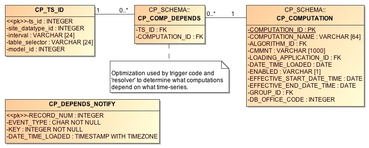
Figure 32: CP_COMP_DEPENDS table used to optimize relationship between time series and computations.

The CP_TS_ID table provides a single unique integer key to a time series. The CP GUIs and the background compproc daemon update this table as needed when new time series are created.

The CP_COMP_DEPENDS table then relates this TS_ID to the computations that must be run when data for this time series is written to HDB. It is the job of the compdepends daemon to keep this table up to date.

The Computation Dependencies Daemon relies on database trigger code and a new table called CP_DEPENDS_NOTIFY. Triggers fire on events that would change the computation dependencies. The trigger places a notification into the CP_DEPENDS_NOTIFY table. The Computation Dependencies Daemon reads the notifications and updates the CP_COMP_DEPENDS table accordingly. The notifications are as follows:

Event Type	Description
T	Time Series Created – a new time series has been created in the database. KEY is the unique database key (i.e. for HDB CP_TS_ID.ts_id). The daemon must check to see if this new time series meets the criteria for a group computation.
D	Time Series Deleted – A time series with the specified KEY was deleted from the database. Any computations depending on this time series will no longer be performed. For group computations, the dependency is simply removed. For single (non-group) computations, the computation itself will be disabled.
M	Time Series Modified – indicates that one of the key fields of a time series has been modified. Dependencies will be re-evaluated.
C	Computation Modified – KEY is the computation ID. Indicates that the specified computation was modified in some way. All previous dependencies are removed and new ones are evaluated.
G	KEY is the time series group ID. Indicates that a time series group was modified. Any computations that use this group (recursively) must be reevaluated.
F	Special message indicating that a full evaluation should be performed. Thus by inserting a record into CP_DEPENDS_NOTIFY with EVENT_TYPE = ‘F’ (e.g. from SQL Developer), you can force a reevaluation of all dependencies.

Interactive Run-Computations GUI

Figure 33 shows the Interactive Run-Computations GUI. The program can be started in two ways:

• Stand-alone from the ‘runcomp’ script in your bin directory.

• Linked to the Computation Editor by pressing the ‘Run Computations’ button as described in section 3.4 above.

When run in stand-alone mode, you select the computations you want to run from a list. When linked to the computation editor, that section of the screen is grayed-out. You are implicitly running the computation-being-edited. Other than this, the operation is the same in both modes.

Just below the computation list, you enter a date/time range and then press the ‘Run Computations’ button. Input values for the selected range are retrieved, the computations are run, and the results are shown in the graph and in the table at the bottom. You can zoom-in/out by dragging and right-clicking the mouse in the graph.

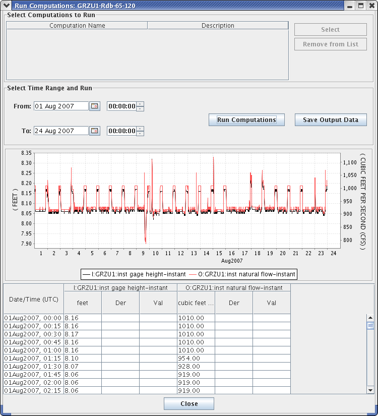
Figure 33: Interactive Run Computations GUI.

Other Utilities

Several other utilities were written as unit-test programs. They may be useful in operational scenarios as well.

List All Computations

Synopsis:

complist

Description:

Prints a list of computations defined in the database.

List All Algorithms

Synopsis:

algolist

Description:

Prints a list of algorithms defined in the database.

List Locks Used by Computation Processes

Synopsis:

complocklist

Description:

Prints a list of computation locks defined in the database. This in essence will give you a list of currently running computation processes.

List the CP_COMP_DEPENDS Table

Synopsis:

decj decodes.tsdb.ShowCompDepends

Description:

This is a trouble-shooting utility to print out the current computation dependencies in a CSV format. The following is an example showing the command and its output for the HDB database. The format for a Time Series Identifier will vary for HDB, Tempest, and CWMS.

decj decodes.tsdb.ShowCompDepends

9936, "TESTSITE1.65.instant.R_", 146, "regtest_006-1-DailyAverage", 50, "compproc_regtest"
9944, "TESTSITE3.65.instant.R_", 146, "regtest_006-1-DailyAverage", 50, "compproc_regtest"
9945, "TESTSITE1.66.day.R_", 147, "regtest_006-2-Disagg", 50, "compproc_regtest"
9946, "TESTSITE3.66.day.R_", 147, "regtest_006-2-Disagg", 50, "compproc_regtest"

The columns are:

• Time Series Key (integer)

• Time Series ID (String – Database Specific Unique Time Series Identifier)

• Computation ID (integer)

• Computation Name (String)

• Computation Process ID (integer)

• Computation Process Name (String)

Output Time Series Data

Synopsis:

outputts [ options ] time-series-ID-1 [ time-series-ID-N … ]

Options:

-F OutputFormat (default=Human-Readable). OutputFormat can be any of the recognized DECODES formatters. See the “rledit” utility, Output Format Enumeration for a list.

-S SinceTime Retrieve data since this time (dd-MMM-yyyy/HH:mm). You can also say “today” for midnight today, “yesterday” for midnight yesterday, or “all” for all data in storage.

-U UntilTime Retrieve data until this time (dd-MMM-yyyy/HH:mm). You can also specify “now”.)

-Z TimeZone Interpret –S and –U arguments in this time zone. Output time-stamps in this time zone.

-G PresentationGrp Apply this DECODES presentation group to the output (sets significant digits and engineering units for each parameter).

In HDB, a Time Series Identifier (TSID) has 4 or 5 parts:

Site.DataType.Interval._R (For Real Data)

Site.DataType.Interval._M.ModelId (For Modeled Data)

For CWMS and OpenTSDB, a TSID has six parts:

Location.Param.ParamType.Interval.Duration.Version

Description:

Retrieves the specified data, formats it, and prints it to the standard output in the specified format.

If you use the “tsimport” format (See TsImport Formatter in the Routing Scheduling Guide), then the output file is compatible with the importts utility described below. This is the easiest way to transfer time series data from one database to another.

Show New Data Assigned to Computations

Synopsis:

compnewdata –a appname

Description:

This is a unit test program to show values created in the CP_COMP_TASKLIST table. It functions in part like the actual computation process:

• Connects to the database as the specified loading app.

• Waits in a loop for task-list records to occur.

• Retrieves and deletes task-list entries

But instead of executing computations, it simply prints the task-list entries to the screen.

We use this utility in the test procedures to clear any unwanted task-list entries before starting a controlled test.

Delete a Time Series

Synopsis:

tsdelete sdi:interval:tabselect:modid

Description:

Deletes last 24 hours worth of data from the specified time series. The time series is identified by a string in the format shown, where:

• sdi = Site Datatype ID

• tabselect = table selector, e.g. “R_”

• modid = model run ID (use -1 for real data)

Import Time Series Data from a File

Synopsis:

importts filename

Description:

Reads the file and imports the data into HDB.

The file has three types of lines:

• SET:TZ=TimeZone

• TSID:Full Time Series Path Name

• Data line: YYYY/MM/DD-HH:MM:SS,Value,Flags

• SET:UNITS=units abbreviation (e.g. “ft”)

The SET and TSID apply to all subsequent data lines.

Evaluate a Time Series Group

To test the group, run the command-line utility showtsgroup:

showtsgroup group-name

The display will show you all information about the group including how it is defined in the database, and an expanded list of all time-series that would currently be considered members of this group.

Convert Individual Computations to Groups (HDB Only)

We have prepared a utility to convert individual computations to group computations. This is intended for USBR offices that have been running old versions of CP and have a sizable number of computations already deployed.

The anticipated workflow is:

1. Prepare a time series group and evaluate it in the “groupedit” GUI. Verify that it contains the time-series you want to use for input for a computation.

2. Prepare a computation that uses the group, but do not yet enable it.

3. Run the utility in test mode and view the report. Verify that the results are what you want.

4. Run the utility again (without test mode). This will enable the group computation and disable any individual computations that are handled by the group.

We provide more detail and examples for each step below.

Prepare Time Series Group

Run the groupedit GUI. Create a group using any of the criteria available. Save the group and press the Evaluate button at the lower right. Verify that the group contains the parameters that you want to use for input to the group computation.

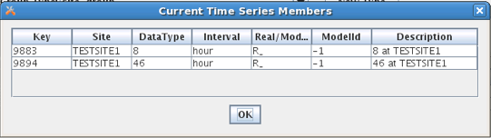
Figure 34: Group Evaluation.

Now suppose we have two individual computations that use the Copy Algorithm to copy these time series values to a modeled (M_) table with model ID 1. One such computation is shown in Figure 35. (Assume that this computation is enabled.)

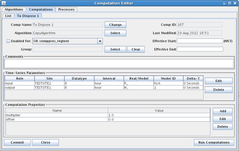
Figure 35: Individual Computation that will be replaced by a group computation.

Prepare a Computation that uses the Group

Now we prepare a computation as shown in Figure 36. Note that the computation is not yet enabled. This will happen when we run the utility.

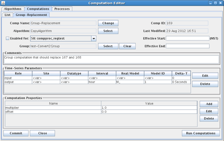
Figure 36: Group Computation that will Replace Individual Computations.

Run the Utility

Synopsis:

convert2group [ options ] Group-Comp-ID

Options:

-T Test Mode. Produce a report of actions to be taken but make no database changes.

-S filename Filename to save disposed computations in. Default is “disposed-comps.xml”

-R filename Filename of the report of actions (to be) taken. Default is “convert2group-report.txt”.

-X delete The default action is to disable computations when they have been replaced by a group. You can use this option to tell the utility to attempt to delete the computation from the database. This will only be successful if there are no data in HDB for these computations. (HDB records the source of every piece of data. It will not let you delete a computation if data exists from it).

The ‘Group-Comp-ID’ is the numeric ID of the new group computation. In our example above it is 169. So to run the utility in test mode, type:

convert2group –T 169

Now examine the report that it produces. Since we did not supply a filename, this is found in “convert2group-report.txt”.

The report will tell us which computations would be affected by the utility, but since we included –T in the command, no actions were actually taken.

If all is well, type the command line again, but without the –T argument.

Following this, reopen compedit. Verify that the individual computations were disabled and the new group-based computation has been enabled.

How the Matching is Done

The Utility expands the group and applies it to the computation input parameters. Then, for each result, it looks for an individual computation with matching input parameters, output parameters, and property settings. If it finds one, the individual computation is a candidate for disposal.

Now consider a special case:

• We have 100 locations with instantaneous stage values.

• We have 100 individual rating computations.

• 99 of them are identical, but one uses different property settings.

• I make a group that specifies instantaneous stage (65) and apply it to a new rating computation.

The utility will find matches for 99 and dispose of 99 individual computations. However the one with different property values will remain enabled. Furthermore the utility will create subgroups so that this input is excluded from the group computation.

Execute Computations over Time Range from Command Line

Synopsis:

compexec options …

Supported options:

-f ControlFileName

• Allows you to use a control file to specify which computations, groups and/or time series to execute. See below.

-S YYYY/MM/dd-HH:mm:ss

• Since time in UTC. If omitted, then all data back to the oldest records in the database are processed.

-U YYYY/MM/dd-HH:mm:ss

• Until time in UTC. If omitted, then all data up to the most recent records in the database are processed.

-C comp

• The comp argument can be either a numeric surrogate key comp-ID or the name of the computation. Both of these are visible in the computation editor on the list panel.

• This option can appear multiple times for multiple computations.

-G group

• group can be either the numeric (surrogate key) time series group ID or the group name. Both are visible in the group editor.

• This option can appear multiple times for multiple groups.

-T TSID

• TSID should be the String Time Series Identifier appropriate for this database.

• This option can appear multiple times for multiple Time Series.

-o OutputFormat

• OutputFormat should be the name of a valid DECODES output formatter.

• Normally this utility will execute the computations and write the results to the time series database. Use this option if you want the results written to the standard output in the specified format, rather than the database. That is, when you use this option, no data will be written back to the database.

-R PresentationGroup

• PresentationGroup should be the name of the DECODES Presentation Group to use.

• This option only takes effect in conjunction with the –o OutputFormat option.

-Z TimeZone

• TimeZone should be the String representation of a valid Java time zone.

• This option only takes effect in conjunction with the –o OutputFormat option.

-q

• This option means quiet mode. No prompts or statistics will be written to the standard output.

Think of specifying -G group as a shortcut to specifying a number of TSIDs with multiple -T arguments. It does not mean to execute only those computations that use the group. It means to evaluate the group into a list of time series IDs and then execute any computation that uses any of those TSIDs as an input.

The -C argument specifies which computations to execute. If a computation is a group-based computation, it could have two meanings:

• If you do NOT also specify time series, it will determine all possible inputs and execute the computation for each possible input set.

• If you DO specify time series, this limits the possible inputs to the named time series.

Which computations, Time Series, and Groups to process are controlled by either the –C, -G, and –T option or in a control file. If you opt to use a control file, it must be an ASCII file in which each line specifies one of the options:

# comment lines begin with ‘#’

tsid ABCDE.Stage.Inst.1Hour.0.Raw

tsid FGHIJ.Stage.Inst.1Hour.0.Raw

group Numeric-Group-Id

comp Numeric-Comp-Id

Examples:

compexec -G AllSpillwayStages -o Human-Readable -S 2016/05/01-12:30:00

Evaluate the group named “AllSpillwayStage” into a set of time series. Then execute any computations that take any of those time series as input. Only use inputs with a since time >= the specified time. Output data to the screen in Human-Readable format.

Note: If you’re not sure what a command is about to do, a good idea is to output it to the screen first and look at the results. If you’re happy, then rerun the command without the -o argument.

compexec -G AllSpillwayStages -S 2016/05/01-12:30:00

Evaluate the group named “AllSpillwayStage” into a set of time series. Then execute any computations that take any of those time series as input. Ingest the results of the computations back into the database.

compexec -G 4 -S 2016/05/01-12:30:00

Evaluate the group with ID=4 into a set of time series. Then execute any computations that take any of those time series as input. Ingest the results of the computations back into the database.

compexec -G 4 -C 27 -C 35 -S 2016/05/01-12:30:00

Evaluate the group with ID=4 into a set of time series. Then execute any computations with ID=27 and ID=35 over the time series in the group. Ingest the results of the computations back into the database.

Features Specific to USBR HDB

The following features apply only to USBR HDB Database.

Model Run ID

This section describes how Model Run ID is handled within computations.

When a computation is triggered by modeled data. The default model run ID for any outputs will be the same as the input.

If the computation was triggered by real data and an output is modeled. The model run ID can be controlled in the following ways:

• The computation processor can be started with the –m argument as described in section 8.1. This becomes the default for all computations.

• The algorithm record can contain a property with name “writeModelRunId”. This will override a default set with the –m argument.

• The computation record can contain a property with name “writeModelRunId”. This will override any default set with –m argument and any property set in the algorithm record.

In a computation has both REAL and MODELED inputs, and it is triggered by only REAL data, the input model run ID will be determined as follows:

• If a property “inputModelRunId” is present, it will be used.

• Otherwise find the most recent model run ID for the specified model ID.

HDB Specific Algorithms

A collection of algorithms were developed for HDB by a separate contractor. These algorithms have come to do the bulk of the computations for USBR. Most of these algorithms provide a thin bridge between the CP infrastructure and the SQL database. The CP is used mainly as a triggering mechanism, the actual computational work is done in database resident procedures.

For OpenDCS 6.2, these legacy algorithms have been included in the “opendcs.jar” release. They are found in the “decodes.algo.hdb” package.

BeginofPeriodAlg

Subsamples a time series by taking the first recorded value within a period.

Note: See the standard Subsample and Resample algorithms described above, which provide more flexibility than this HDB-specific algorithm.

Time Series Parameters:

Role Name	Type	Description
input	input	The input time series.
output	output	The time series output. The Interval of the output parameter determines the aggregate period.

Properties:

Property Name	Java Type	D efault	Description
re q_window_period	int	0	See below. If the first input value is not within the specified number of periods, then do NOT output the value.
desire d_window_period	int	0	See below. If the first input value is not within the specified number of periods, then flag the output with validation flag ‘w’.
validation_flag	String	<empty>	Specify validation flags for all output values.

The definition of the two ‘window period’ properties depends on the interval of the output parameter:

• If the output parameter is HOUR, then the parameter is a number of minutes.

• If the output parameter is DAY, then the parameter is a number of hours.

• If the output parameter is MONTH, then the parameter is a number of days.

• If the output parameter is YEAR or WY, then the parameter is a multiple of 31 days.

In all cases, if the period is 0 (the default) then the check is not done.

CallProcAlg

Takes up to 5 input values labeled input1 … input5. Uses these to call a procedure named in the callproc property.

Time Series Parameters:

Role Name	Type	Description
input1…input5	input	The input time series parameters.
output	output	This is a dummy output parameter and is never set by the algorithm. The procedure specifed by the proccall property would have to set any outputs directly.

Properties:

Property Name	Java Type	D efault	Description
proccall	String	(none)	The complete procedure call containing masks <<input1>> … <<input5>> masks representing the input parameters. You can also include a mask <<tsbt>> representing the time slice base time.

DynamicAggregatesAlg

Note: See the ‘Stat’ algorithm described in section 5.25. Stat provides a more efficient and portable way of performing many of the functions described here.

This algorithm performs aggregation across HDB intervals. It can do any Oracle-based aggregation that takes a single input time series. The ‘aggregate_name’ property specifies which function to call, which can be any of the following:

• min

• max

• avg

• count

• sum

• median

• stddev

• variance

Time Series Parameters:

Role Name	Type	Description
input	input	The input time series.
output	output	The time series output. The Interval of the output parameter determines the aggregate period.

Properties:

Property Name	Java Type	D efault	Description
agregate_name	String	(none)	The name of the Oracle aggregate function.
min_values_required	int	1	No output is produced if there are fewer than this many inputs in the aggregate period. See description below of min-value processing for months.
min_values_desired	int	0	If fewer than this many inputs are present then the output is flagged as a “partial” calculation.
partial_calculations	b oolean	false	If true, then partial calculations are accepted, but are flagged at ‘T’ (Temporary)

Min-Value Processing for Months

If min_values_required or min_values_desired is zero or negative and the output interval is MONTH, then it means that the value is actually the number of input intervals that is allowed to be missing. For example, suppose input interval is DAY and output interval is MONTH, and we are calculating the aggregate for June, which has 30 days. The following table contains examples.

min_val ues_required	min_val ues_desired	partial_c alculations	# days pre sent	r esult?
-1	0	false	29	Yes
-1	0	false	28	No
-5	-1	true	28	Yes – ‘T’
-5	-1	false	28	No

End Of Period Algorithm

Note: See the standard Subsample and Resample algorithms described above, which provide more flexibility than this HDB-specific algorithm.

Output the last value seen within an aggregate period.

Time Series Parameters:

Role Name	Type	Description
input	input	The input time series. for the aggregate period are aggregated by the specified Oracle function.
output	output	The time series output.

Properties:

Property Name	Java Type	D efault	Description
req_windowperiod	i nteger	0	If >0, then this represents the maximum number of input intervals from the end of period in which there must be a value. Example: input=hour, output=day, req_window_period=3. Then an output is produced only if an input is present within the last 3 hours of the day.
desired_window_period	i nteger	0	Like req_window_period, but an output can still be produced, but it will be flagged with the supplied validation flag.
validation_flag	String	(empty)	If an output is produced, but it is outside of the desired window period, it will be flagged with this validation flag.

EOPInterpAlg (End Of Period Interpolating)

Note: See the standard Resample algorithm above which provides more flexibility for resampling and interpolating than the HDB-specific algorithm described here.

This algorithm uses the same inputs, outputs, and properties as described above for End Of Period Algorithm. The only difference is that if the actual value at the end of the period is missing, it will be interpolated.

EquationSolverAlg

Takes up to 5 input values labeled input1 … input5. Uses these to construct a SQL query as specified in the ‘equation’ property. The output value will be set to the result of the equation.

Time Series Parameters:

Role Name	Type	Description
input1…input5	input	The input time series parameters.
output	output	Will be set to the result of the equation.

Properties:

Property Name	Java Type	D efault	Description
equation	String	(none)	The complete procedure call containing masks <<input1>> … <<input5>> masks representing the input parameters. You can also include a mask <<tsbt>> representing the time slice base time. As of 6.7 RC02, the following substitutions are also made: <<loading_application_id>>, <<computation_id>>, <<algorithm_id>>
validation_flag	String	(none)	If specified, the validation flag is set to the first character of the supplied string.

FlowToVolumeAlg

This algorithm calculates volume by aggregating interval flows over time. The output interval determines the time.

Time Series Parameters:

Role Name	Type	Description
input	input	The input flow
output	output	The output volue.

Properties:

Property Name	Java Type	D efault	Description
partial_calculations	b oolean	false	Set to true to allow output when only part of the period is known.
observations_calculation	b oolean	false
min_values_required	i nteger	1	Number of input values required before output can be made. Zero means all.
min_values_desired	i nteger	0	If specified number of inputs is not present, then ‘w’ validation flag will be set.
flow_factor	String	864 00/43560	Use as a multiplier for flow-to-volume calculation.
validation_flag	String	(none)	If specified, the validation flag is set to the first character of the supplied string.

The bulk of the work for computing aggregates is done by SQL functions in the hdb_utilities package. The following query is used:

select hdb_utilities.get_sdi_unit_factor(inputSDI) *

hdb_utilities.get_sdi_unit_factor(outputSDI) * flow_factor *

day_multiplier * average_flow volume ,

hdb_utilities.date_in_window(’outputInterval’,

to_date(’_aggregatePeriodBegin’,’dd-MM-yyyy HH24:MI’))

is_current_period from dual;

HdbACAPSRating

Type: Time-Slice

Implements the ACAPS rating algorithm from tables in the database. Independent value is “elevation”. Dependent values are “storage” and “area”.

Parameters:

Name	Type Code	Description
elevation	input	Reservoir elevation in ft.
storage	output	Storage in cubic feet
area	output	Area in acre-feet

HdbEvaporation

Type: Time-Slice

This algorithm uses an input area time series to compute evaporation from a coefficient that is dependent on the area. The coefficient can be provided as a second time series input, or, if it is not provided or not present at this time slice, a lookup value will be used from one of the stat tables in HDB. Ideally, a coefficient time series should be provided that incorporates temperature and relative humidity.

The state table is:

• R_intervalSTAT for real values, where interval is the interval of the area time series.

• M_intervalSTAT for modeled values

Parameters:

Name	Type Code	Description
area	input	Area or average area over period in acre-feet.
evapCoeff	input	Coefficient Time Series in ft/day
evap	output	Evaporation in acre-feet

Properties:

Name	J ava Typ e	De fault	Description
ignoreTimeSeries	B ool ean	false	If set to true, then ignore the evapCoeff time series, even if it is provided. Always look up the evaporation coefficient from the HDB stat table.

HdbRating Algorithm

Type: Time-Slice

Important: If you have upgraded from a previous version of CP, you may have the wrong Algorithm record. Open compedit, click the Algorithms Tab, Open the HdbShiftRating algorithm. Make sure the executable class is (exactly) as follows:

decodes.tsdb.algo.HdbShiftRating

Parameters:

Name	Java Type	Type Code	Description
indep	double	i (simple input)	The independent value to be rated.
dep	double	output	The rated (e.g. flow) value.

Properties:

Name	** Java Ty pe**	De fault	Description
exceedLowerBound	Boolean	false	Set to true to allow rating to extend the rating below the lowest value of the table. May be invalid for certain rating types.
exceedUpperBound	Boolean	false	Set to true to allow rating to extend the rating above the highest value of the table. May be invalid for certain rating types.
ratingType	String	Shift A djusted Stage Flow	This property provides the HDB_TABLE type for the actual rating table, which indirectly determines the lookup algorithm.
applyShifts	Boolean	false	If true, add the ‘shift’ property value before table lookup.
shift	double	0	Constant shift value added to indep before look, but only if applyShifts == true.

Description:

The output (dep) value is:

dep = ratingTable.lookup(indep) # if applyShifts == false

or

dep = ratingTable.lookup( indep + shift ) # if applyShifts == true

HdbShiftRating Algorithm

Type: Time-Slice

Important: If you have upgraded from a previous version of CP, you may have the wrong Algorithm record. Open compedit, click the Algorithms Tab, Open the HdbShiftRating algorithm. Make sure the executable class is (exactly) as follows:

decodes.hdb.algo.HdbShiftRating

Parameters:

Name	Java Type	Type Code	Description
indep	double	i (simple input)	The independent value to be rated.
dep	double	output	The rated (e.g. flow) value.
shift	double	output	The shift used at this timeslice.

Properties:

Name	Java Type	Def ault	Description
variableShift	Boolean	false	False means to use a constant shift value provided by the “singleShift” property. True means to use a separate lookup table for shifts.
singleShift	double	0	If variableShift == false, which is the default, then this property provides the single shift value to be used for all time slices.
shiftTableType	String	Stage Shift	if variableShift is set to True, then a separate table is used to lookup a shift value at each time slice. This property provides the HDB_TABLE type.
lookupTableType	String	Stage Flow	This property is new in OpenDCS 6.3. In previous releases it was hard-coded to “Stage Flow”. This property provides the HDB_TABLE type for the actual rating table.

Description:

At each time slice, a shift is determined. If variableShift==false, the shift is constant. Else the shift is looked up by applying the indep stage value to a separate Shift table. The shift value is available as an output. The output (dep) value is:

dep = ratingTable.lookup( indep + shift )

InflowAdvancedAlg

Type: Time-Slice

The output is simply the sum of all of the non-missing input values. A preferred method of doing this would be to use the standard ScalarAdder algorithm.

This algorithm is an Advanced mass balance calculation for inflow as:

Delta Storage + Total Release + Delta Bank Storage + evaporation

• all incoming diversions + all outgoing diversions

If any of the input properties are set to “fail” then the inflow will not be calculated and/or the inflow will be deleted. If all of the inputs do not exist because of a delete the inflow will be deleted if the output exists regardless of the property settings.

Class Name: decodes.hdb.algo.InflowAdvancedAlg

Parameters:

Name	Type Code	Description
total_release	input
delta storage	input
inflow	output

InflowBasicAlg

Type: Time-Slice

The output is simply the sum of all of the non-missing input values. A preferred method of doing this would be to use the standard ScalarAdder algorithm.

This algorithm is an Advanced mass balance calculation for inflow as:

Delta Storage + Total Release + Delta Bank Storage + evaporation

• all incoming diversions + all outgoing diversions

• (up to 5 diversions of each type)

If any of the input properties are set to “fail” then the inflow will not be calculated and/or the inflow will be deleted. If all of the inputs do not exist because of a delete the inflow will be deleted if the output exists regardless of the property settings.

Class Name: decodes.hdb.algo.InflowAdvancedAlg

Parameters:

Name	Type Code	Description
total_release	input
delta_storage	input
delta_bs	input	bank storage
evap	input
diver_in1 … 5	input	Up to 5 diversion inputs. Unused ones should be set to MISSING=Ignore in the Computation Parameter Dialog
diver_out1 … 5	input	Likewise
inflow	output

PowerToEnergyAlg

PowerToEnergyALg - calculates Energy base on power readings converted to hourly Megawatt rates.

Input Time Series:

• input

Output Time Series:

• output

Properties:

• partial_calculations: boolean: default false: if current period partial calculations will be performed

• min_values_required: number: default 1: the minimum number of observations required to perform computation

• min_values_desired: number: default 0: the minimum number of observations desired to perform computation

• validation_flag: string: default empty: the validation flag value to be sent to the database

This algorithm uses the hdb_utilities.get_sdi_unit_factor SQL function.

SideInflowAlg

This algorithm is an Side Inflow mass balance calculation for inflow as: Delta Storage - Total Release Above + Total Release Below + evaporation.

If inputs Delta Storage, or Total Release Above, or Total Release Below, or if the Evap do not exist, or have been deleted, and if the Delta_STORAGE_MISSING, or the TOTAL_REL_ABOVE_MISSING, or EVAP_MISSING, or TOTAL_REL_BELOW_MISSING properties are set to “fail” then the inflow will not be calculated and/or the inflow will be deleted. If all of the inputs do not exist because of a delete the inflow will be deleted if the output exists regardless of the property settings.

This algorithm written by M. Bogner, August 2008 Modified by M. Bogner May 2009 to add additional delete logic and version control

Input Time Series:

• delta_storage

• evap

• total_rel_above

• total_rel_below

Output Time Series:

• side_inflow

VolumeToFlowAlg

VolumeToFlowAlg calculates average flows based on the sum of the inputs volumes for the given period:

• Flow (cfs) = sum of volumes * 43560 sq ft per acre / # of days / 86400 seconds

This algorithm assumes units are in cfs and acre-feet; if not a conversion is done to output the correct units

Properties:

• partial_calculations: boolean: default false: if current period partial calculations will be performed

• min_values_required: number: default 1: the minimum number of observations required to perform computation

• min_values_desired: number: default 0: the minimum number of observations desired to perform computation

• validation_flag: string: default empty: the validation flag value to be sent to the database

• flow_factor: Number: use as multiplier for volume to flow factor (.5,.5041) : Default: 43560/86400

Input Time Series:

• input

Output Time Series:

• output

HDB Site Specific Algorithms

In addition to the above algorithms, there are several site specific HDB algorithms:

• BMDCUnreg – Blue Mesa Unregulated Inflow

• CRRCUnreg – Crystal Unregulated Inflow

• EstGLDAInflow – computes Lake Powell inflow from the three upstream gages

• FLGUUnreg – Flaming Gorge Unregulated Inflow

• GLDAEvap – Lake Powell Evaporation

• GLDAUnreg – Lake Powell Unregulated Inflow

• GlenDeltaBSMBaAlg – Glen Canyon Bank Storage Mass Balance

• ParshallFlume – Stage to Flow computation for Parshall Flume

Features Specific to CWMS

Rating Tables within the CWMS Database

The following utilities are included for working with Rating objects inside the CWMS database:

listRatings List all of the rating objects in the database.

importRating Import a rating from an XML file.

exportRating Export a rating to an XML file.

editRatings A GUI for listing, viewing, importing, and exporting ratings.

In each case, type the command with a –x argument to have it list available options.

Virtual Gage Algorithm

Type: Time-Slice

Input Parameters:

Name	Java Type	Type Code
upstreamGage	double	i
downstreamGage	double	i

Output Parameter:

virtualGage : double precision

Properties:

Name	Java Type	Default
upstreamPosition	double	0.0
downstreamPosition	double	10.0
virtualPosition	double	5.0
upstreamGageZero	double	0.0
downstreamGageZero	double	0.0
virtualGageZero	double	0.0

Description:

Compute a virtual elevation at an intermediate point between two other gages.

Inputs are the upstream and downstream elevation,

Properties specify Upstream position (e.g. Mile number), Downstream position, and Virtual Gage position.

The positions are required to do proper interpolation. Default values place the virtual gage halfway between up & downstream gages.

If provided, you may set gage-zero properties for each of the locations, thus the output can be in gage height or elevation.

Validation with DATCHK Files

Algorithm Name: DatchkScreening

Type: Time-Slice

Input Parameters:

Name	Java Type	Type Code
input	double	i

Output Parameter:

output : double precision (optional – see below)

Properties:

Name	Java T ype	Def ault	Meaning
noOverwrite	Boolean	False	If set to true, then don’t overwrite output values that already exist at a given time. Can only be used if the input and output refer to different time series.
setInputFlags	Boolean	False	If set to true, then set the flag bits on the input parameter in addition to the output parameter. Can only be used if the input and output refer to different time series.
setRejectMissing	Boolean	False	If set to true, then if the validation results in the value being rejected, then write a dummy output value with flags indicating that it is MISSING. Can only be used if the input and output refer to different time series.
noOutputOnReject	Boolean	False	If set to true and the output time series is different from the input, then when a value is flagged as REJECTED as the result of validation, do not write any value to the output.

Description:

This algorithm performs validation and sets flag values in the output (and optionally, the input) parameter. The validation information is stored in files for the legacy DATCHK utility that worked with DSS.

The CCP DATCHK implementation can do the following types of checks:

• Absolute Magnitude – Compare input value with constant min/max values.

• Duration Magnitude – Accumulate value over defined period and then check it against constant min/max. Typically used for incremental precip.

• Constant Value – Check to see if a value has remained constant (within a given tolerance) over a specified time period.

• Rate of Change (per Hour) – Check min/max rate of change per hour.

For a complete description of the checks see the legacy DATCHK manual, typically called CPD-65.pdf, available for download at a number of USACE sites.

The DATCHK Validation algorithm will set flag bits on the input parameter directly. You can optionally have it copy the value to another time series, along with the resulting flag bits, by setting an output parameter in the computation. If the output parameter is left undefined, then only the input flags are set.

Results of Validation

Validation results can be stored on every time series value in your CWMS database. Currently a 32-bit integer is used to store all results in a compact form. Figure 37 shows the bit layout.

The CWMS user should not need to care about the internal representation of flag bits. This section is included for completeness and technical reference only.

  3                   2                   1
2 1 0 9 8 7 6 5 4 3 2 1 0 9 8 7 6 5 4 3 2 1 0 9 8 7 6 5 4 3 2 1
P - - - - - T T - T - T T T T T T M M M M C C C D R R V V V V S
|           <---------+---------> <--+--> <-+-> | <+> <--+--> |
|                     |              |      |   |  |     |    +------Screened T/F
|                     |              |      |   |  |     +-----------Validity Mutually-Exclusive Flags
|                     |              |      |   |  +--------------Value Range Integer
|                     |              |      |   +-------------------Different T/F
|                     |              |      +---------------Replacement Cause Integer
|                     |              +---------------------Replacement Method Integer
|                     +-------------------------------------------Test Failed Mutually-Exclusive Flags
+-------------------------------------------------------------------Protected T/F

Figure 37: CWMS Time Series Value Quality Flags.

After a value is screened by the validation algorithm, the ‘S’ (low order) bit will be set.

The four bits labeled “VVVV” can take on the following values:

• 0 = Unknown validity

• 1 = Validity OK (all screening tests passed)

• 2 = Missing

• 4 = Questionable

• 8 = Rejected

If the Protected (high order) bit is set in the output value, it will not be modified in any way by the validation algorithm.

The several bits labeled ‘T’ indicate which test failed, e.g. ABSOLUTE_MAGNITUDE, RATE_OF_CHANGE, etc.

DATCHK Configuration Files

Top Config File

The CCP Algorithm reads a top-level configuration file telling where to find the DATCHK files and other mapping files. By default, this top-level configuration file is called “datchk.cfg” and is stored in your $DECODES_INSTALL_DIR. You can modify the location by setting the “datchkConfigFile” property in the toolkit setup menu (or the “decodes.properties” file).

The top config file is a simple XML file. An example is shown below.

<DatchkConfig>

<!– The pathmap file maps DSS paths to CWMS paths –>

<pathmap>./pathmap.txt</pathmap>

<!– One or more datchk files go here –>

<datchk>./TESTSITE2.datchk</datchk>

</DatchkConfig>

Pathmap File

The pathmap file maps DSS Path Names to CWMS Time Series IDs. It also supplies the engineering units that are used in the DATCHK criteria definitions.

The pathmap file contains lines in the following format:

CwmsTimeSeriesID=DSS-PATH;Units=unit-abbr;…other assignments

where…

• CmwsTimeSeriesId is a valid CWMS Time Series ID. This is the time series to be validated.

• DSS-PATH is the DSS Path name used in the DATCHK files for this time series

• unit-abbr is a valid CCP Engineering Unit abbreviation. This specifies the units used in DATCHK file criteria definition.

• Other assignments are possible on this line for legacy reasons. They are ignored.

Examples:

TESTSITE1.Flow.Inst.0.0.test=/TEST/TESTSITE1/FLOW//1HOUR/OBS;Units=cfs

TESTSITE1.Precip.Inst.0.0.test=/TEST/TESTSITE1/PRECIP///OBS;Units=in

DATCHK Criteria Files

The format for DATCHK Criteria Files is defined in DATCHK & DATVUE Data Screening Software User’s Manual, February 1995. It is distributed as CPD-65.pdf from HEC.

Several DATCHK Criteria files may be specified in the Top Config File. The definitions are loaded and combined.

At the time of this writing the only CRITERIA types that are supported are:

• ABS – Absolute Magnitude

• DUR – Duration Magnitude

• CONST – Constant Value Checks

• RATE – Hourly Rate of Change Checks

As of OpenDCS 6.1 RC08 we have extended the functionality of DUR and CONST to support irregular time series (ABS could already support irregular).

For CONST checks, one extension was needed to the syntax: The last argument on the line is described in the HEC document as “nmiss”, meaning the maximum number of contiguous missing values allowed in the period being checked. It defaults to zero. If there are more than this number of contiguous missing values in the period, the check is aborted.

For irregular time series there is no way to determine whether a value was expected and therefore missing. Consequently, for irregular time series, you may use any valid CWMS interval (e.g. 4Hours, 2Days) instead of a number. This represents the maximum allowable amount of time between values in the period.

Example:

CRITERIA CONST Q 2D 0.0 0.1 12Hours

This means to check for a constant value (within a tolerance of .1) over the past 2 days, but if there is more than 12 hours between contiguous values in the period, abort the check.

Rating Algorithm for a Single Independent Value

Algorithm Name: CwmsRatingSingleIndep

Type: Time-Slice

Input Parameters:

Name	Java Type	Type Code
indep	double	i

Output Parameter:

dep : double precision

Properties:

Name	Java Type	Default
specVersion	String	“Production”
templateVersion	String	“USGS-EXSA”
useDepLocation	Boolean	false
locationOverride	String	none

Description:

This algorithm performs a rating using rating tables stored within the CWMS database.

A “Rating Specification” in CWMS is specific to a location and parameters at that location. For a rating with a single independent parameter, a Rating Specification ID is a string of the form:

LocationID . IndepParam ; DepParam . TemplateVersion . SpecVersion

For example, a Stage/Flow rating at site BMD might be:

BMD.Stage;Flow.USGS-EXSA.Production

CP builds the specification ID from the information provided:

• Location is normally taken from the independent time series used as input. If the ‘useDepLocation’ property is set to true, the location from the output ‘dep’ param will be used.

  • If locationOverride property is supplied, then it is used to determine the location. This supports wildcards in a similar manner to the location portion of a time series parameter TSID.

• Indep and Dep Param values come from the input and output time series provided

• TemplateVersion and SpecVersion are provided as properties, which can be specified either in the algorithm or computation records.

Rating Algorithm for Multiple Independent Values

Algorithm Name: CwmsRatingMultiIndep

Type: Time-Slice

Input Parameters:

Name	Java Type	Type Code	MISSING action
indep1	double	i	Fail
indep2	double	i	Ignore
indep3	double	i	Ignore
indep4	double	i	Ignore
indep5	double	i	Ignore
indep6	double	i	Ignore
indep7	double	i	Ignore
indep8	double	i	Ignore
indep9	double	i	Ignore

Output Parameter:

dep : double precision

Properties:

Name	Java Type	Default
specVersion	String	“Production”
templateVersion	String	“USGS-EXSA”
useDepLocation	Boolean	false
locationOverride	String	Use this to directly specify the location for the rating spec, or to apply a wildcard (*) mask to either the indep1 or dep (if UseDepLocation is set) location

Description:

This algorithm performs a rating using rating tables stored within the CWMS database. It can handle up to 9 independent time series inputs.

See the discussion above in the previous section (Single Independent) about constructing a Rating Specification ID. The only difference here is that there can be multiple DepParam strings, separated by semicolons. For example a rating with 3 dependent variables with parameters Elev, Gate1, and Gate2 might be:

BMD.Elev;Gate1;Gate2.NAE-Derived.Production

The location for the specification is normally taken from the first independent parameter (which is required). If the ‘useDepLocation’ property is set to true, then the location will be taken from the output dep parameter.

As of 6.3 RC05 the locationOverride property may be used to modify the location (either indep1 or dep, if useDepLocation is true). If it contains wildcard (*) characters, the mask is applied in the same manner that the location part of a time series parameter is applied for a group computation.

The algorithm allows up to 9 independent parameters, but most ratings only take a small number. You should delete any “indepN” parameters you don’t need from the computation record. For example, Figure 38 shows the computation editor screen for a rating with three independent parameters. Note that “indep4” through “indep9” have been deleted.

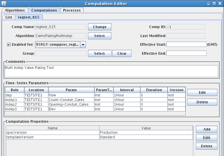
Figure 38: Computation Editor showing Rating with Three Independent Parameters.

Figure 39: Param List for a Computation with Three Independent Parameters.

Make sure you change the Missing-Action for the defined parameters to something other than “Ignore”:

• FAIL: Do not produce an output (dep) if this independent parameter is missing at this time.

• PREV: Use the previous value for this independent parameter if it is missing at this time.

• NEXT: Use the next value for this independent parameter if it is missing at this time.

• INTERP: Interpolate between previous and next if if this independent parameter is missing at this time.

• CLOSEST: Use the closest value (in time) for this independent parameter if it is missing at this time.

Figure 40 shows the dialog for the indep3 parameter (Elev). We have chosen FAIL.

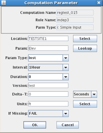
Figure 40: Computation Parameter Dialog, Showing the ‘FAIL’ setting for Independent Parameter 3.

If you are using CWMS Parameter values for the first time, you may encounter a popup telling you to enter the new parameters into the DECODES database editor, presentation tab. For example, when we first entered the computation for a multi-variable rating using conduit gates we had to add these parameters. We entered them into our “CWMS-English” Presentation group, as shown in Figure 41. Be sure to also enter the appropriate units for the new parameters.

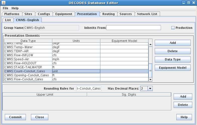
Figure 41: Entering new Parameter Values into the CWMS-English Presentation Group.

CWMS Parameters and DECODES Data Types

DECODES allows data types from many different standard systems such as SHEF, USGS, CWMS, and HDB. DECODES stores data types in a table that includes columns Standard, Code.

CWMS ‘Parameters’ are mapped to DECODES data types with the standard ‘CWMS’.

There are places in the DECODES and CCP GUIs where a list of data types (a.k.a. Parameter) values are presented for the user to select from. We have prepared a utility you can run at any time to copy all CWMS Parameter values so that they are visible to DECODES and CP. Run this utility with the following command:

decj decodes.cwms.CwmsParam2DataType

It may be necessary to re-run this utility from time to time as your CWMS database is populated with Parameter values outside of the CCP.

Validation from CWMS Screening Database

As of OpenDCS 6.2 RC13 the CP can do validations from screening records stored in the CWMS Database. This section will:

• Explain the CWMS screening records,

• Describe tools for importing, exporting, and editing the records,

• Describe the Cwms Screening Algorithm

CWMS Screening Database Records

The CWMS CMA web utility provides the capability for you to create, view, edit, and delete screening records. This section will provide a brief overview of the information therein. The logical arrangement of screening records is depicted in Figure 42.

• Each time series may be assigned to a single screening. Note that CWMS CMA also assigns a resulting TSID. This is not supported by CCP because output parameters are specified by the CCP infrastructure already.

• Each screening has a unique 16 character ID (name)

• Each screening may have multiple seasons. A season is denoted by the start month and day. A season starts at midnight on the specified day in the time zone associated with the time series location.

• Each criteria record (season) may have multiple Duration/Magnitude checks, each denoted by a different duration.

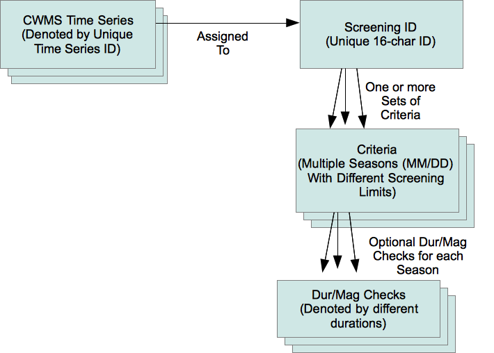
Figure 42: Logical Arrangement of CWMS Screening Records.

The criteria records contain limits that are used for screening the time series values. These are modeled on the screening operations available in DATCHK. As a result of screening, the quality bits associated with each time series value will be set to Good, Questionable, or Rejected.

The checks include:

• Absolute Range Check: Low/High limits are set for Questionable and Rejected.

  • Example: if Stage > 13.5, flag the value as questionable.

• Hourly Rate of Change Check: Rise/Fall limits are set for Questionable and Rejected

  • Example: If Stage has risen more than 6 inches per hour, flag the value as questionable.

• Constant Value (e.g. stuck sensor): Checks whether a sensor value has remained constant (within a specified tolerance) over a specified time period.

  • Example: If Precip has not changed more than .1 inch for the 5 days, flag the value as questionable

• Duration/Magnitude Checks accumulate values over a specified duration and then allow you to specify limits. They are designed for cumulative precip.

  • Example: If there has been more than 14.5” of rain in the past 12 hours, flag the value as questionable.

Each type of check may be independently enabled or disabled. For example, you may disable all of the constant value checks associated with a screening ID, but allow all the other checks to proceed.

Importing DATCHK Screening Information

As a convenience for districts that are already using DATCHK screening, we have provided a utility to import DATCHK screening records. See the section above on DATCHK Screening for a discussion of how these screening tests are specified. They involve three types of files:

• The overall DATCHK Configuration File

• Path Map files map CWMS Time Series IDs to DSS Path Names

• Crit files contain the DATCHK criteria. A file may be optionally assigned to a season.

The utility is started as follows:

datchkImport [-C] datchk-config-file

The –C argument means to confirm each screening before it is written to the database. It is a good idea to include this argument.

The datchk-config-file argument is required. In your DATCHK algorithm, this is normally set by the DECODES property called ‘datchkConfigFile’.

The utility will read all of the pathmap and crit files specified in the configuration file into memory, along with the assignments to time series. Then it will write the criteria records to the database. If you specified the –C argument it will ask permission before writing each one.

Now recall that each screening ID must have a unique 16-character ID. The DATCHK files do not specify the screening ID so the import program must construct one. It does so as follows:

6-chars-location . 4-chars-param . 4-char-hash

That is, the first 6 chars of the location, followed by the first 4 chars of the Param, followed by a 4-character hash code of the entire Time Series ID (used to guarantee uniqueness).

For example, the screening for WVD.Stage-Tailwater.Inst.15Minutes.0.DCP-raw will be named “WVD.STAG.ibVK”.

The CWMs CMA web application allows you to rename the screenings and assign multiple time series to the same screening after the import.

Export Screening Information

Synopsis:

screeningExport [-n *screeningId*] [-q] [-G *presgrp*] [-A] [-E] [-T *tsid*]

…where:

-n screeningId Output a specific screening by its unique name

-q Query the user for a list of screening IDs

-G presgrp Apply the specified presentation group to the screening limits, allowing you to control the precise units in the export file.

-A Export All of the screenings. This is useful as a backup mechanism

-E Export screenings in English units (default is SI).

-T tsid Output the screening for the specified time series identifier.

Screenings are exported in a plain text format as depicted below. Information is printed to the standard output. You can redirect to a file to capture the output. For example, to take a backup of all your screenings in English units to a file called “screenings.bak”:

screeningExport –A –E >screenings.bak

Note that the CRITERIA records are identical to DATCHK criteria files

SCREENING unique-16-char-ID

DESC Several lines may be included here

DESC with the complete description of the screening.

PARAM CWMS Param ID, e.g. Stage-Pool

PARAMTYPE CWMS Param Type ID, e.g. Inst

DURATION CWMS Duration ID, e.g. 0

UNITS The CWMS Units ID used to specify the limits

RANGE_ACTIVE true or false

ROC_ACTIVE true or false

CONST_ACTIVE true or false

DURMAG_ACTIVE true or false

CRITERIA_SET

SEASON MM/DD, e.g. 03/21 for a season that starts on March 21

CRITERIA … Multiple Criteria records as they appear in a DATCHK file

CRITERIA_SET_END

other criteria sets can appear here for a screening with multiple seasons.

ASSIGN CWMS-Time-SeriesId : Screening ID.

Here is an example screening with two seasons and four time series assigned to it:

SCREENING regtest_027

PARAM Flow

PARAMTYPE Inst

DURATION 0

UNITS cfs

RANGE_ACTIVE true

ROC_ACTIVE true

CONST_ACTIVE true

DURMAG_ACTIVE true

CRITERIA_SET

SEASON 1/1

CRITERIA ABS R 4 20

CRITERIA ABS Q 8 16

CRITERIA RATE Q -1.5 1.5

CRITERIA CONST Q 2D 0 0 3

CRITERIA_SET_END

CRITERIA_SET

SEASON 1/2

CRITERIA ABS R 2 22

CRITERIA ABS Q 4 20

CRITERIA RATE Q -1.5 1.5

CRITERIA CONST Q 2D 0 0 3

CRITERIA_SET_END

SCREENING_END

ASSIGN TESTSITE2.Flow.Inst.1Hour.0.test : regtest_027

ASSIGN TESTSITE3.Flow.Inst.1Hour.0.test : regtest_027

ASSIGN TESTSITE4.Flow.Inst.1Hour.0.test : regtest_027

ASSIGN TESTSITE1.Flow.Inst.1Hour.0.test : regtest_027

Importing Screening Records

A utility is provided to import record from screening files described in the previous section. This provides you a way to edit screening records outside of the CWMS CMA GUI:

• Export desired screening records to a file.

• Make modifications with a text editor.

• Import the modified records.

Synopsis

screeningImport [-T] [y] screening-files …

… where:

• -T means do NOT import time series assignments. Only import screening records.

• -y means to import screenings without asking for confirmation. The default behavior is to ask for confirmation before each screening is written.

The Screening Algorithm

The CWMS Screening Algorithm is called “CwmsScreening”. You may need to import the screening algorithm one time before using:

compimport $DCSTOOL_HOME/imports/comp-cwms/CwmsScreeningAlgorithm.xml

You will now see the Screening Algorithm in the Algorithms tab of the computation editor. It will also be in the selection list for algorithms when you are creating computations.

The screening algorithm is designed to work the same way as the DATCHK Screening algorithm described above in section 12.3. The properties are the same. You are encouraged to read that section for details.

The only difference between the algorithms is where the screenings are read:

• DATCHK Screening opens the specified datchk.config file to load path map files and criteria files.

• CWMS Screening reads screening information from the CWMS database.

CWMS Screening Editor

As of OpenDCS 6.1 RC15, the package includes a GUI Editor for CWMS Screening Records. The GUI is not yet integrated with the Launcher Button bar. To start it, use the script:

screeningEdit

It takes the normal options that other OpenDCS programs take, like:

• -l logfilename

• -d1, -d2, -d3 to set the debug level

The initial screen is a tabbed pane with two tabs. The Screening IDs tab shows a list of all screening IDs that exist in your database:

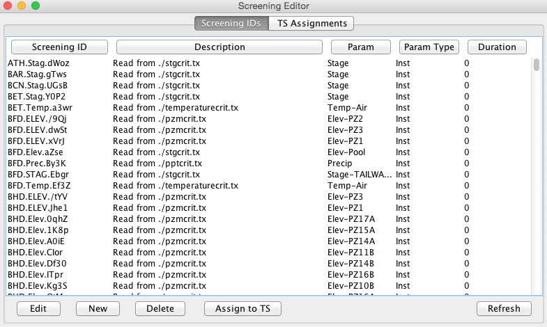
You can sort the list in various ways by clicking the column headers. Use the buttons at the bottom to:

• Edit: Open a selected screening to modify its seasons, limits, etc.

• New: Create a new screening.

• Delete: Delete one or more selected screenings.

• Assign to TS: Assign a selected screening to one or more Time Series IDs.

• Refresh: Re-read the list from the database

The TS Assignments tab shows you all current time series assignments to screenings:

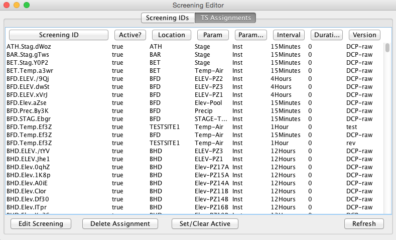
Again, you can sort the list by clicking the column headers. Use the buttons at the bottom to:

• Edit Screening: Open the screening ID on a selected line to modify its seasons, limits, etc.

• Delete Assignment: Delete the assignments for one or more selected lines. Note that this deletes the assignment to time series. It does not delete the screening ID.

• Set/Clear Active: In CWMS, a screening record can be made inactive. You can select one or more lines and then press this button to change the Active setting.

• Refresh: Re-read the list from the database.

When you open a screening ID for edit, you get a new tab (it works just like the DECODES database editor):

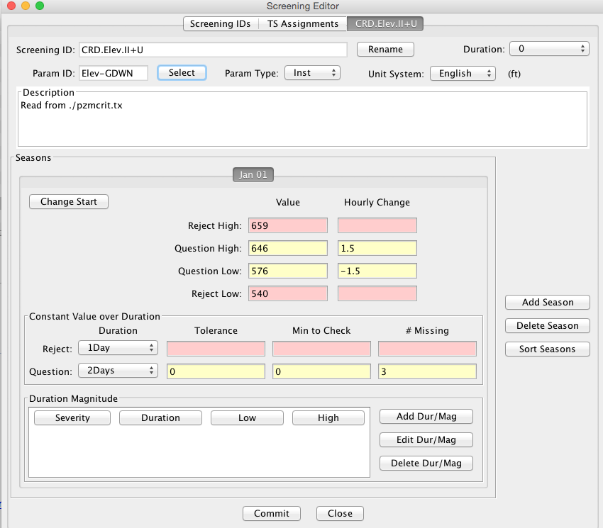
The header area of this screen allows you to:

• Rename the Screening ID – The system will verify that the new name is unique.

• Set the Duration for this screening with a pull-down list.

• Select the Param ID for this screening from a list of known parameter IDs in your database.

• Select the Param Type (Total, Ave, Inst, Max, Min) from a pull-down list.

• Select the Unit System that you want to use for viewing and editing limit values. The system looks up the appropriate units for the Param ID you have selected and shows it next to the Unit System pull-down.

• Type a multi-line description.

The footer is just like the DECODES editor. You can Commit any changes you have made and then Close the tab.

The middle area of the screen shows the “Seasons” for this Screening ID. All screenings must have at least one Season, which by default starts on Jan 1. Each Season allows you to specify a start date and a different set of screening criteria.

Reject limits are highlighted in red, Questionable limits in yellow. Hover over any of the fields to get a tooltip with a detail explanation of what the control does.